Transformations of the FEP/FES

Once a free energy profile/surfaces has been constructed in terms of a collective variable CV, we can transform it a posteriori to another free energy profiles in terms of another CV. This can be done in two different ways, depending on the nature of the relation between old and new CV:

Deterministic transformation from free energy $F_1(CV)$ to free energy profile $F_2(Q)$ with a deterministic relation described by the mathematical function $Q=f(CV)$
Probabilistic transformation from free energy $F_1(CV)$ to free energy profile $F_2(Q)$ with a probabilistic relation described by the conditional probability $P(Q|CV)$

Deterministic transformation

1 dimensional

Once a free energy profile has been constructed in terms of a collective variable CV, it can be transformed a posteriori to a free energy profile in terms of a new collective variable Q that is mathematical function of the original CV, in other words $Q=f(CV)$ . This is based on the transformation of variables in probability theory:

$F_2(Q) &= F_1(f^{-1}(Q)) - k_B T \log\left[\frac{df^{-1}}{dQ}(Q)\right] \\ &= F_1(f^{-1}(Q)) + k_B T \log\left[\frac{df}{dCV}(f^{-1}(Q))\right]$

To do such transformation in ThermoLIB, we need two things: (1) the original free energy profile (FEP) $F(CV)$ and (2) a function $Q=f(CV)$ and optionally its derivative (if the derivative is not given, it will be estimated through numerical differentiation) to encode the relation between old and new collective variable. The original FEP is defined by an instance of the BaseFreeEnergyProfile class (or of its child classes). The function $Q=f(CV)$ (and its derivative) can be defined as a simple python routine. To illustrate lets consider the function 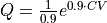$Q=\frac{1}{0.9}e^{0.9\cdot CV}$ , which we can define in python as follows:

def function(cv):
    return np.exp(0.9*cv)/0.9

def derivative(cv):
    return np.exp(0.9*cv)

Using this, we can perform the transformation from the old FEP fep to the new FEP fep_new as follows:

fep_new = fep.transform_function(function, derivative=derivative)

Note

Specifying the derivative is optional. If not specified, ThermoLIB will estimate it through numerical differentation.

2 dimensional

In case of a transformation of a 2D free energy surface, this can be generalized as followed. Assuming a transformation formula of the form:

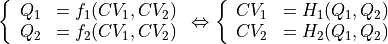
$\left\{\begin{array}{rl} Q_1 &= f_1(CV_1,CV_2) \\ Q_2 &= f_2(CV_1,CV_2) \\ \end{array}\right. \Leftrightarrow \left\{\begin{array}{rl} CV_1 &= H_1(Q_1,Q_2) \\ CV_2 &= H_2(Q_1,Q_2) \end{array}\right.$

with $(H_1,H_2)$ the inverse of $(f_1,f_2)$ . The transformed free energy surface $F_Q(Q_1,Q_2)$ is given by:

$F_Q(Q_1,Q_2) &= F_{CV}(H_1(Q_1,Q_2),H_2(Q_1,Q_2)) + k_B T \log\left[J\left(H_1(Q_1,Q_2),H_2(Q_1,Q_2)\right)\right]$

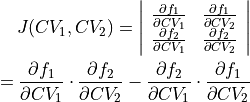
where $J(CV_1,CV_2)$ represents the Jacobian determinant of the transformation:

$J(CV_1,CV_2) = \left|\begin{array}{cc} \frac{\partial f_1}{\partial CV_1} & \frac{\partial f_1}{\partial CV_2} \\ \frac{\partial f_2}{\partial CV_1} & \frac{\partial f_2}{\partial CV_2} \end{array}\right| \\ = \frac{\partial f_1}{\partial CV_1}\cdot\frac{\partial f_2}{\partial CV_2} - \frac{\partial f_2}{\partial CV_1}\cdot\frac{\partial f_1}{\partial CV_2}$

To do such transformation in ThermoLIB, we again need the transformation formulas $f_1(CV_1,CV_2)$ and $f_2(CV_1,CV_2)$

f1 = lambda x,y: np.sqrt(2)/2*(x-2.75+y+1.25)
f2 = lambda x,y: np.sqrt(2)/2*(y+1.25-x+2.75)

However, now it is also mandatory to specify the new grid in $(Q_1,Q_2)$ space.

bins_q1 = np.arange(-1.2,1.4+0.025,0.025)
bins_q2 = np.arange(-1.0,1.0+0.025,0.025)

Using this input, we can apply the transform_function method as follows

fes_new = fes.transform_function((f1,f2), bins_q1, bins_q2, cv1_label='Q1', cv2_label='Q2')

Probabilistic transformation

Consider the situation of two collective variables CV and Q which are not deterministically related, in other words there is not a unique relation between the two. However, there is a the stochastic correlation between the two, which means we can determine the conditional probability $P(Q|CV)$ expressing the probability to find the system in a state with a specific value of Q given that is already is in a state with specific value of CV. This information can be used to transform the free energy profile $F_1(CV)$ towards $F_2(Q)$ using Bayes theorem from probability theory:

$F_2(Q) &= -k_B T \log\left[\int P(Q|CV)\cdot e^{-\beta F_1(CV)} dCV\right]$

To do so, we first determine the conditional probability $P(Q|CV)$ using the ConditionalProbability1D1D class as follows:

#initialize conditional probability
condprob = ConditionalProbability1D1D()

#initialize TrajectoryReaders to extract CV and Q values from trajectory files
cv_reader = ColVarReader([0])
q_reader  = ColVarReader([1])

#Read trajectory files and extract samples for conditional probability
for i in range(ntraj):
    condprob.process_simulation(
        [('COLVAR_%i.dat' %i, q_reader)],
        [('COLVAR_%i.dat' %i, cv_reader)],
    )

#Compute conditional probability in given bin ranges
bins_cv = np.arange(start, end, width)
bins_q = np.arange(start, end, width)
condprob.finish([bins_q], [bins_cv])

Finally, the original FEP can be tranformed to the new FEP as follows:

fep_new = condprob.transform(fep)

Note

One can verify that even if there is a deterministic relation $Q=f(CV)$ , but we would still do the probabilistic transformation, we get the same result as if we would have done the deterministic transformation.

Mathematically, this can be proven by realizing that a deterministic relation of the form $Q=f(CV)$ can be interpreted as an extreme case of stochastic correlation with conditional probability given by $P(Q|CV)=\delta(Q-f(CV))$ , in which $\delta$ represents the Dirac delta function/distribution.

Numerically this can be illustrated by using the two approaches given above using the routines implemented in ThermoLIB.