Tutorial 4 - Advanced techniques in error estimation

Introduction

In this notebook, we investigate the impact of sample correlation on the error estimate of free energy profiles in ThermoLIB. To this end, we will discuss the ussage of the decorrelate routine and its under-the-hood corrtime_from_acf routine, including various interesting optional features. Furthermore, we consider various alternative ways (such as block averaging and bootstriding) of constructing free energy profiles to attempt to estimating error bars and compare the results at the end.

[1]:

%load_ext autoreload
%autoreload 2

[2]:

from thermolib.thermodynamics.fep import SimpleFreeEnergyProfile, plot_profiles
from thermolib.thermodynamics.histogram import Histogram1D, plot_histograms
from thermolib.tools import read_wham_input, blav, decorrelate, corrtime_from_acf
from thermolib.thermodynamics.trajectory import ColVarReader
from thermolib.units import *

import numpy as np, matplotlib.pyplot as pp

[3]:

prefix = 'advanced_wham1D_error_'

Impact correlation between samples on FEP

In this section, we illustrate the impact of correlation between subsequent samples in the MD trajectories. To that end, we apply a regular WHAM procedure to all biased simulation data defined in data/wham_input.txt using all trajectory samples, as well as using only a sample every 10/100/1000 steps.

[4]:

bins = np.arange(-1.6, 1.6, 0.02)
fn_meta = 'data/formic_acid_dimer/wham_input.txt'

[5]:

colvar_reader_1 = ColVarReader([0], units=['au'])
temp, biasses, trajectories_1 = read_wham_input(
    fn_meta, colvar_reader_1, 'colvars/correlated/COLVAR_%s.dat',
    bias_potential='Parabola1D', q01_unit='au', kappa1_unit='kjmol',
)
hist_1 = Histogram1D.from_wham(bins, trajectories_1, biasses, temp, error_estimate='mle_f', Nscf=10000)
fep_1 = SimpleFreeEnergyProfile.from_histogram(hist_1, temp=temp)

WARNING: the CV range you specified for the histogram does not cover the entire simulation range in trajectory 127. Simulation samples outside the given CV range were cropped out.
SCF Converged!
---------------------------------------------------------------------
TIMING SUMMARY
  initializing: 00h 00m 00.000s
  histograms  : 00h 00m 00.167s
  bias poten. : 00h 00m 00.009s
  solve scf   : 00h 00m 00.203s
  error est.  : 00h 00m 00.574s
  TOTAL       : 00h 00m 00.955s
---------------------------------------------------------------------

[6]:

colvar_reader_10 = ColVarReader([0], stride=10 ,units=['au'])
temp, biasses, trajectories_10 = read_wham_input(
    fn_meta, colvar_reader_10, 'colvars/correlated/COLVAR_%s.dat',
    bias_potential='Parabola1D', q01_unit='au', kappa1_unit='kjmol',
)
hist_10 = Histogram1D.from_wham(bins, trajectories_10, biasses, temp, error_estimate='mle_f', Nscf=10000)
fep_10 = SimpleFreeEnergyProfile.from_histogram(hist_10, temp=temp)

WARNING: the CV range you specified for the histogram does not cover the entire simulation range in trajectory 127. Simulation samples outside the given CV range were cropped out.
SCF Converged!
---------------------------------------------------------------------
TIMING SUMMARY
  initializing: 00h 00m 00.000s
  histograms  : 00h 00m 00.017s
  bias poten. : 00h 00m 00.006s
  solve scf   : 00h 00m 00.149s
  error est.  : 00h 00m 00.345s
  TOTAL       : 00h 00m 00.519s
---------------------------------------------------------------------

[7]:

colvar_reader_100 = ColVarReader([0], stride=100 ,units=['au'])
temp, biasses, trajectories_100 = read_wham_input(
    fn_meta, colvar_reader_100, 'colvars/correlated/COLVAR_%s.dat',
    bias_potential='Parabola1D', q01_unit='au', kappa1_unit='kjmol',
)
hist_100 = Histogram1D.from_wham(bins, trajectories_100, biasses, temp, error_estimate='mle_f', Nscf=10000)
fep_100 = SimpleFreeEnergyProfile.from_histogram(hist_100, temp=temp)

SCF Converged!
---------------------------------------------------------------------
TIMING SUMMARY
  initializing: 00h 00m 00.000s
  histograms  : 00h 00m 00.003s
  bias poten. : 00h 00m 00.006s
  solve scf   : 00h 00m 00.375s
  error est.  : 00h 00m 00.471s
  TOTAL       : 00h 00m 00.857s
---------------------------------------------------------------------

[8]:

colvar_reader_1000 = ColVarReader([0], stride=1000 ,units=['au'])
temp, biasses, trajectories_1000 = read_wham_input(
    fn_meta, colvar_reader_1000, 'colvars/correlated/COLVAR_%s.dat',
    bias_potential='Parabola1D', q01_unit='au', kappa1_unit='kjmol',
)
hist_1000 = Histogram1D.from_wham(bins, trajectories_1000, biasses, temp, error_estimate='mle_f', Nscf=10000)
fep_1000 = SimpleFreeEnergyProfile.from_histogram(hist_1000, temp=temp)

SCF Converged!
---------------------------------------------------------------------
TIMING SUMMARY
  initializing: 00h 00m 00.000s
  histograms  : 00h 00m 00.001s
  bias poten. : 00h 00m 00.006s
  solve scf   : 00h 00m 00.453s
  error est.  : 00h 00m 00.515s
  TOTAL       : 00h 00m 00.976s
---------------------------------------------------------------------

[9]:

plot_profiles([fep_1000,fep_100,fep_10,fep_1], labels=['stride=1000', 'stride=100', 'stride=10', 'stride=1'], flims=[0,40])

<Figure size 640x480 with 0 Axes>

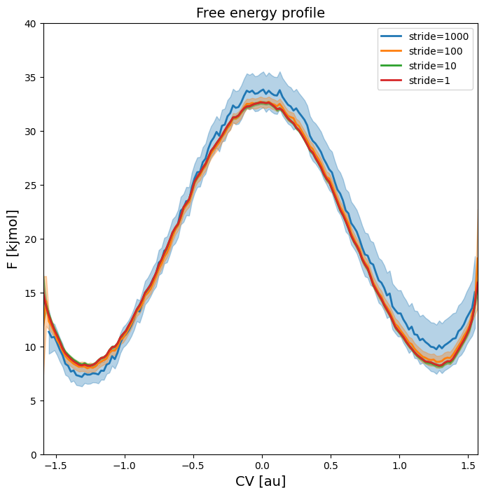
../_images/tut_advanced_error_estimation_14_1.png

The plot above indicates that the error becomes larger as the stride increases (which is logical as it gives WHAM a lot less data to work with). We also observe that the (mean) estimated free energy itself becomes more noisy as the stride increases, which is also due to lower number of samples.

Estimating the autocorrelation time

The question now is which is the most reliable representation of the error. To that end, we estimate the correlation time from the autocorrelation function of the collective variable itself during the trajectories. We first illustrate this for a few individual trajectories:

[10]:

corrtime = corrtime_from_acf(trajectories_1[8], plot=True, xlims=[0,5000], ylims=[-1.05,1.05])

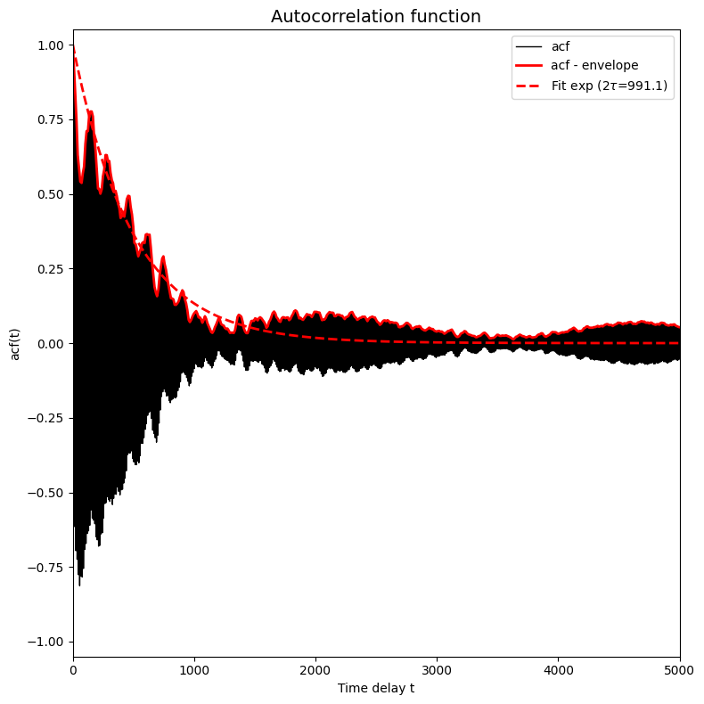
../_images/tut_advanced_error_estimation_18_0.png

In this plot the black solid line (which became a solid black region because it is a very fast oscilling curve, see further) represents the autocorrelation function, the red solid line represents the envoloppe of the black curve/region and the red dashed curve presents a fit of $\exp(-\frac{t}{\tau})$ to the red solid curve.

The above plot is an example of a typical situation in which the trajectory contains atomistic vibrations that happen on a very small time scale. These vibrations are responsible for the very high frequency oscillations you see in the plot above (resulting in the seemingly solid black region). If we want to fit a simple exponential function (to estimate the time decay constant which is the correlation time), we cannot fit directly to the curve itself as it fluctuates equally between above and below zero and hence any fit will give flat curve. Instead, we first filter out the very high frequency oscillations by computing the enveloppe of the curve. This is done by default in the corrtime_from_acf routine given the default value n_nested_envelopes=1, but can be switched off by means of setting n_nested_envelopes=0.

In some cases, it is usefull to indeed switch this off. For example when you did a simulation in which you did not print out every time step, but only every so many time steps resulting in a time series that do not contain these high frequency oscillations any more. In other situations it might be the case the enveloppe still contains such oscillations that make fitting difficult, then you can compute the enveloppe of the enveloppe by setting n_nested_envelopes=2. Below, we show what happens if we put n_nested_envelopes=2 for the current case.

[11]:

ct = corrtime_from_acf(trajectories_1[8], plot=True, xlims=[0,5000], ylims=[-1.05,1.05], n_nested_envelopes=2)
print('Fitted (integrated) correlation time: 2*tau =  %.3f timesteps' %ct)

/home/lvduyfhu/miniconda3/envs/test/lib/python3.14/site-packages/thermolib/tools.py:960: OptimizeWarning: Covariance of the parameters could not be estimated
  pars, pcovs = curve_fit(function, upper_envelope_indices, upper_envelope_values, **curve_fit_kwargs)

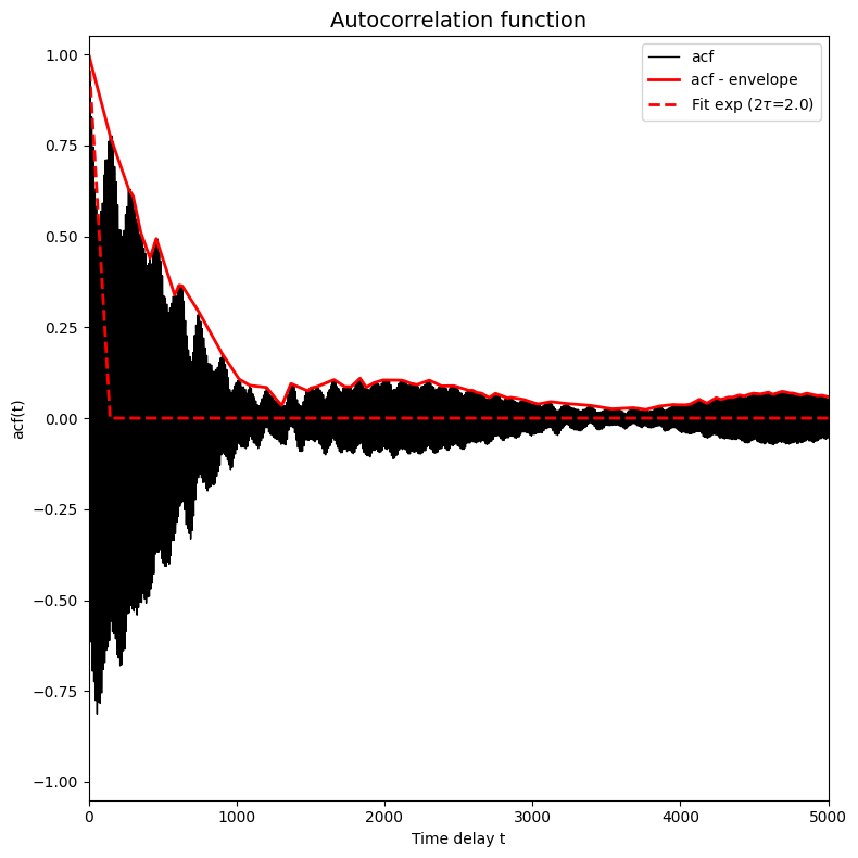
../_images/tut_advanced_error_estimation_20_1.png

Fitted (integrated) correlation time: 2*tau =  2.000 timesteps

You indeed see that the enveloppe contains even less oscillations. However, a new problem arises, a problem that also might have arissen from the start (e.g. again when the simulation only printed out every so many steps). This new issue is that the fit (dashed red line) is very bad. In fact, a closer look to the resulting correlation time reveals that no fit was done at all. Indeed we see that the integrated correlation time equals $2\cdot\tau=2$ or hence $\tau=1$ . This is just the initial guess of $\tau$ (which is by default set to 1) is returned. Therefore, we need to adjust the initial gues of the correlation time $\tau$ to a better value, which we can do with the keyword p0. If we would make another bad guess, i.e. set the initial gues to 2, we will still be confronted with the same issue. Let us first illustrate that by indeed setting the initial guess to 2:

[12]:

ct = corrtime_from_acf(trajectories_1[8], plot=True, xlims=[0,5000], ylims=[-1.05,1.05], n_nested_envelopes=2, p0=[2])
print('Fitted (integrated) correlation time: 2*tau =  %.3f timesteps' %ct)

../_images/tut_advanced_error_estimation_22_0.png

Fitted (integrated) correlation time: 2*tau =  4.000 timesteps

We now again clearly see a bad fit, which is also again reflected by the fact that the result $2\cdot\tau=4$ (hence $\tau=2)$ just returns the initial guess. In order to make a better initial gues, we can just look at the plot of the red solid line. We clearly see that the initial decay happens on a time scale of 1000 timesteps, so we could just use that as initial guess:

[13]:

ct = corrtime_from_acf(trajectories_1[8], plot=True, xlims=[0,5000], ylims=[-1.05,1.05], n_nested_envelopes=2, p0=[1000])
print('Fitted (integrated) correlation time: 2*tau =  %.3f timesteps' %ct)

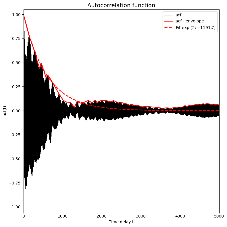
../_images/tut_advanced_error_estimation_24_0.png

Fitted (integrated) correlation time: 2*tau =  1191.743 timesteps

Which now indeed represents a much better fit. The above discussion is included here to highlight what might happen when computing correlation times and how to try and adress those issues. In the present case, however, the default settings of n_nested_enveloppe=1 and p0=[1] is just fine and we therefore proceed with those default settings.

Constructing the FEP with correlated error estimate

Let us now compute the correlation time for each trajectory. This can be done using the decorrelate routine. In this routine, we can also adjust the parameters for the enveloppe and the initial conditions by specifying respectively the n_nested_envelopes and p0 arguments. However, in the following we can use the default values.

[14]:

corrtimes = decorrelate(trajectories_1, plot=True)

<Figure size 640x480 with 0 Axes>

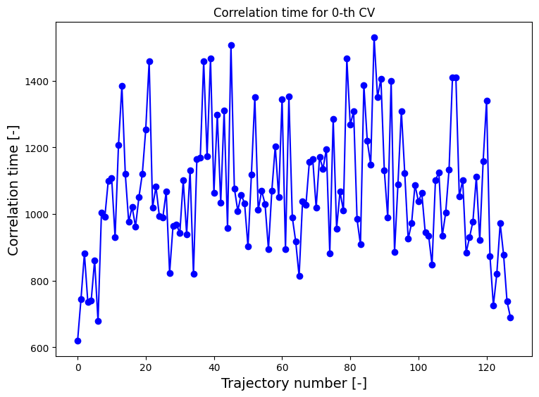
../_images/tut_advanced_error_estimation_28_1.png

The above routine returns the correlation times for each simulation (i.e. each umbrella). As the error estimation is based on the Fisher information matrix of the maximum likelihood estimator, we can reconstruct the free energy profile using all original samples, but now we also parse the correlation times to the from_wham routine to obtain a more reliable error estimation by accounting for the reduced information due to correlation (i.e. only $\frac{N}{2\cdot\tau-1}$ independent samples instead of $N$ ) in the information matrix:

[15]:

hist_decor = Histogram1D.from_wham(bins, trajectories_1, biasses, temp, error_estimate='mle_f', corrtimes=corrtimes, Nscf=10000)
fep_decor = SimpleFreeEnergyProfile.from_histogram(hist_decor, temp=temp)
#fep_decor.set_ref(ref='min')

WARNING: the CV range you specified for the histogram does not cover the entire simulation range in trajectory 127. Simulation samples outside the given CV range were cropped out.
SCF Converged!
---------------------------------------------------------------------
TIMING SUMMARY
  initializing: 00h 00m 00.000s
  histograms  : 00h 00m 00.160s
  bias poten. : 00h 00m 00.011s
  solve scf   : 00h 00m 00.192s
  error est.  : 00h 00m 00.459s
  TOTAL       : 00h 00m 00.823s
---------------------------------------------------------------------

[16]:

plot_profiles([fep_decor,fep_1], labels=['MLE-decor', 'MLE-naive'], flims=[0,40])

<Figure size 640x480 with 0 Axes>

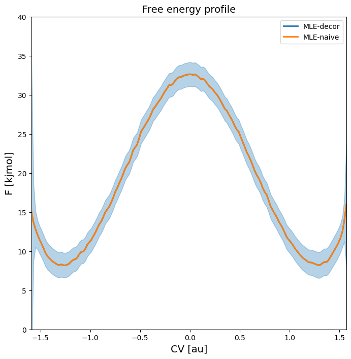
../_images/tut_advanced_error_estimation_31_1.png

We indeed see that the error bar increases from almost zero (for the case of assuming all samples to be independent, i.e. correlation time equal to 0) to a value of around 1-2 kJ/mol based on the correlation time.

Evaluating the correlated error estimate

In order to test the above error estimation, we are now going to generate profiles from various sources of subsets of the original trajectories and investigate whether the WHAM profile generated by each subset indeed falls within the predicted error bar. In order to make a fair comparison in terms of the error bar, we will make sure that each method uses trajectories that have approximately a number of samples equal to 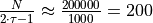$\frac{N}{2\cdot\tau-1}\approx\frac{200000}{1000}=200$ , i.e. the previously estimated number of uncorrelated samples in a trajectory. The various methods for generating subsets of data are:

Delayed-strided profiles: subset starting at sample 0, 100, 200, … and with with a sampling stride of 1000
Blocked profiles: subset [0,200], [200,400], …
Bootstrapped profiles: subsets each containing 200 random samples

Delayed-strided WHAM profiles

[18]:

starts = np.arange(0,1000,100)
feps = []
for start in starts:
    print("Constructing WHAM FEP for start=%i" %start)
    colvar_reader = ColVarReader([0], units=['au'], start=start, stride=1000)
    temp, biasses, trajectories = read_wham_input(
        fn_meta, colvar_reader, 'colvars/correlated/COLVAR_%s.dat',
        bias_potential='Parabola1D', q01_unit='au', kappa1_unit='kjmol',
    )
    hist = Histogram1D.from_wham(bins, trajectories, biasses, temp, Nscf=10000)
    fep = SimpleFreeEnergyProfile.from_histogram(hist, temp)
    #fep.set_ref(ref='min')
    feps.append(fep)

Constructing WHAM FEP for start=0
SCF Converged!
---------------------------------------------------------------------
TIMING SUMMARY
  initializing: 00h 00m 00.000s
  histograms  : 00h 00m 00.001s
  bias poten. : 00h 00m 00.007s
  solve scf   : 00h 00m 00.456s
  error est.  : 00h 00m 00.000s
  TOTAL       : 00h 00m 00.465s
---------------------------------------------------------------------
Constructing WHAM FEP for start=100
SCF Converged!
---------------------------------------------------------------------
TIMING SUMMARY
  initializing: 00h 00m 00.000s
  histograms  : 00h 00m 00.001s
  bias poten. : 00h 00m 00.006s
  solve scf   : 00h 00m 00.384s
  error est.  : 00h 00m 00.000s
  TOTAL       : 00h 00m 00.392s
---------------------------------------------------------------------
Constructing WHAM FEP for start=200
SCF Converged!
---------------------------------------------------------------------
TIMING SUMMARY
  initializing: 00h 00m 00.000s
  histograms  : 00h 00m 00.001s
  bias poten. : 00h 00m 00.005s
  solve scf   : 00h 00m 00.393s
  error est.  : 00h 00m 00.000s
  TOTAL       : 00h 00m 00.401s
---------------------------------------------------------------------
Constructing WHAM FEP for start=300
SCF Converged!
---------------------------------------------------------------------
TIMING SUMMARY
  initializing: 00h 00m 00.000s
  histograms  : 00h 00m 00.001s
  bias poten. : 00h 00m 00.006s
  solve scf   : 00h 00m 00.470s
  error est.  : 00h 00m 00.000s
  TOTAL       : 00h 00m 00.479s
---------------------------------------------------------------------
Constructing WHAM FEP for start=400
SCF Converged!
---------------------------------------------------------------------
TIMING SUMMARY
  initializing: 00h 00m 00.000s
  histograms  : 00h 00m 00.001s
  bias poten. : 00h 00m 00.007s
  solve scf   : 00h 00m 00.155s
  error est.  : 00h 00m 00.000s
  TOTAL       : 00h 00m 00.164s
---------------------------------------------------------------------
Constructing WHAM FEP for start=500
SCF Converged!
---------------------------------------------------------------------
TIMING SUMMARY
  initializing: 00h 00m 00.000s
  histograms  : 00h 00m 00.001s
  bias poten. : 00h 00m 00.006s
  solve scf   : 00h 00m 00.341s
  error est.  : 00h 00m 00.000s
  TOTAL       : 00h 00m 00.349s
---------------------------------------------------------------------
Constructing WHAM FEP for start=600
SCF Converged!
---------------------------------------------------------------------
TIMING SUMMARY
  initializing: 00h 00m 00.000s
  histograms  : 00h 00m 00.002s
  bias poten. : 00h 00m 00.006s
  solve scf   : 00h 00m 00.482s
  error est.  : 00h 00m 00.000s
  TOTAL       : 00h 00m 00.490s
---------------------------------------------------------------------
Constructing WHAM FEP for start=700
SCF Converged!
---------------------------------------------------------------------
TIMING SUMMARY
  initializing: 00h 00m 00.000s
  histograms  : 00h 00m 00.001s
  bias poten. : 00h 00m 00.006s
  solve scf   : 00h 00m 00.425s
  error est.  : 00h 00m 00.000s
  TOTAL       : 00h 00m 00.433s
---------------------------------------------------------------------
Constructing WHAM FEP for start=800
SCF Converged!
---------------------------------------------------------------------
TIMING SUMMARY
  initializing: 00h 00m 00.000s
  histograms  : 00h 00m 00.001s
  bias poten. : 00h 00m 00.005s
  solve scf   : 00h 00m 00.287s
  error est.  : 00h 00m 00.000s
  TOTAL       : 00h 00m 00.294s
---------------------------------------------------------------------
Constructing WHAM FEP for start=900
SCF Converged!
---------------------------------------------------------------------
TIMING SUMMARY
  initializing: 00h 00m 00.000s
  histograms  : 00h 00m 00.001s
  bias poten. : 00h 00m 00.006s
  solve scf   : 00h 00m 00.367s
  error est.  : 00h 00m 00.000s
  TOTAL       : 00h 00m 00.375s
---------------------------------------------------------------------

[19]:

fep_delstr = SimpleFreeEnergyProfile.from_average(feps, error_estimate='std')
plot_profiles([fep_decor]+feps, labels=['MLE-decor']+['start=%i' %start for start in starts], flims=[0,40],
               colors    =['k']+[None,]*len(starts),
               linewidths=[2  ]+[1   ,]*len(starts),
               linestyles=['-']+['--',]*len(starts))

<Figure size 640x480 with 0 Axes>

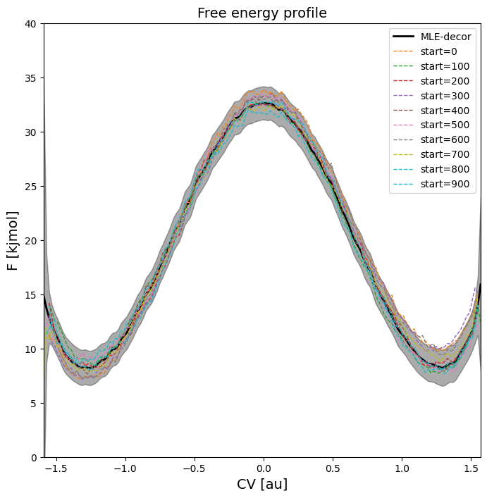
../_images/tut_advanced_error_estimation_37_1.png

All profiles indeed fall within the predicted 2-sigma error bar.

Blocked WHAM profile

Here, for each original trajectory, a new trajectory is constructed in which each subsequent block of 1000 samples is replaced by its average.

[20]:

blocksize = 1000
nblocks = int(min([len(traj) for traj in trajectories_1])/blocksize)
new_trajs = []
for itraj, trajectory in enumerate(trajectories_1):
    new_traj = np.zeros(nblocks)
    for i in range(nblocks):
        new_traj[i] = trajectory[i*blocksize:(i+1)*blocksize].mean()
    new_trajs.append(new_traj)
hist_block = Histogram1D.from_wham(bins, new_trajs, biasses, temp)
fep_block = SimpleFreeEnergyProfile.from_histogram(hist_block, temp)

SCF did not converge!
---------------------------------------------------------------------
TIMING SUMMARY
  initializing: 00h 00m 00.000s
  histograms  : 00h 00m 00.001s
  bias poten. : 00h 00m 00.006s
  solve scf   : 00h 00m 00.056s
  error est.  : 00h 00m 00.000s
  TOTAL       : 00h 00m 00.064s
---------------------------------------------------------------------

[21]:

plot_profiles([fep_decor,fep_block], labels=['MLE-decor','block'], flims=[0,40],
                colors=['k',None], linestyles=['-','--'], linewidths=[3,1])

<Figure size 640x480 with 0 Axes>

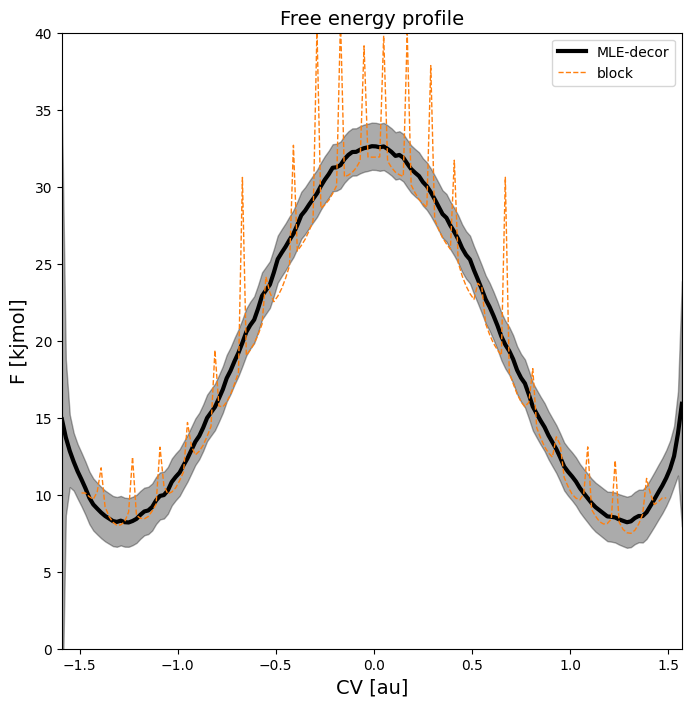
We see that the block profile is within the error predicted by the decorrelated profile, except for the many spikes. These spikes are due to the severaly overlap between subsequant umbrella trajectories after averaging. To illustrate lets consider the histograms of 3 subsequent original trajectories as well their blocked counterparts:

[22]:

bins2 = np.arange(-0.25,0.251,0.01)
hists = [
    Histogram1D.from_single_trajectory(trajectories[61],bins2),
    Histogram1D.from_single_trajectory(trajectories[62],bins2),
    Histogram1D.from_single_trajectory(trajectories[63],bins2),
    ]
labels = ['61-orig', '62-orig', '63-orig', ]
plot_histograms(hists, labels=labels, linestyles=['-','-','-'], colors=['r','b','g'])

<Figure size 640x480 with 0 Axes>

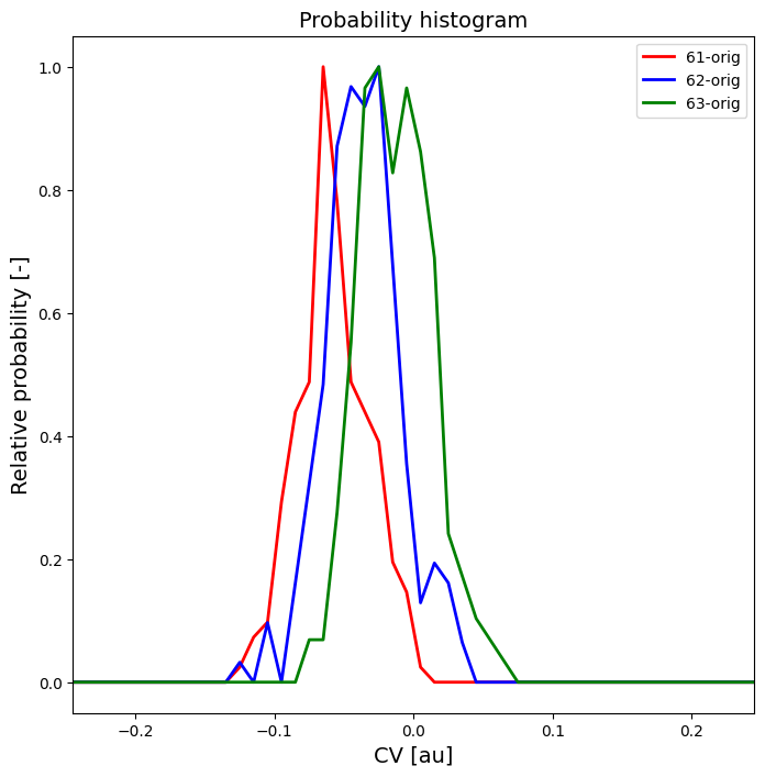
The above plot clearly shows sufficient overlap in the original trajectories.

[23]:

hists = [
    Histogram1D.from_single_trajectory(new_trajs[61],bins2),
    Histogram1D.from_single_trajectory(new_trajs[62],bins2),
    Histogram1D.from_single_trajectory(new_trajs[63],bins2),
    ]
labels = ['61-block', '62-block', '63-block']
plot_histograms(hists, labels=labels, linestyles=['-','--','--'], colors=['r','b','g'])

<Figure size 640x480 with 0 Axes>

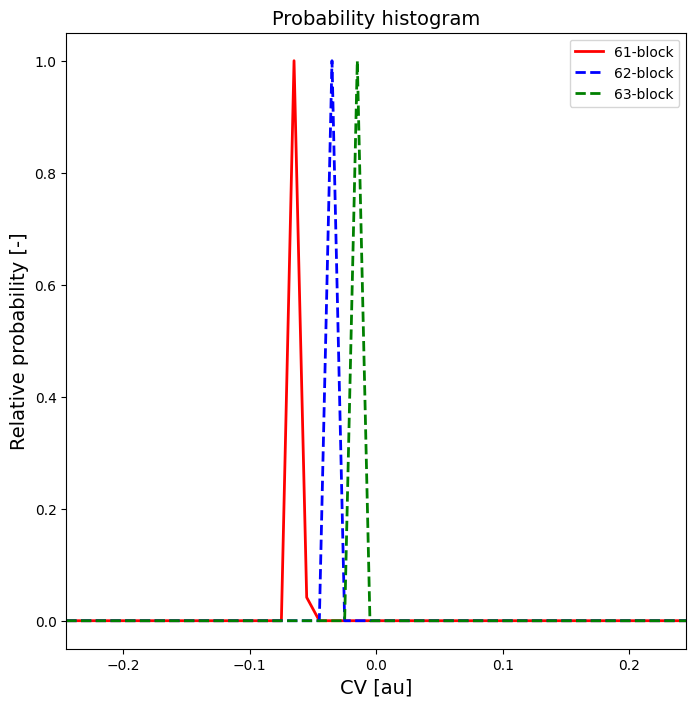
The above plot clearly shows a lack of overlap in the new trajectories.

Bootstrapped WHAM profiles

Finally, we again reconstruct various FEPS, but know using bootstrapping applied to each of the original biased simulations. Again, we consider 10 trajectories.

[24]:

Nboot = 10
size = 200
feps3 = []
for iboot in range(Nboot):
    new_trajectories = []
    for traj in trajectories_1:
        Nsteps = len(traj)
        indices = np.random.randint(0, high=Nsteps, size=size)
        new_trajectories.append(traj[indices])
    hist = Histogram1D.from_wham(bins, new_trajectories, biasses, temp, Nscf=10000)
    fep = SimpleFreeEnergyProfile.from_histogram(hist, temp)
    feps3.append(fep)

SCF Converged!
---------------------------------------------------------------------
TIMING SUMMARY
  initializing: 00h 00m 00.000s
  histograms  : 00h 00m 00.001s
  bias poten. : 00h 00m 00.011s
  solve scf   : 00h 00m 00.203s
  error est.  : 00h 00m 00.000s
  TOTAL       : 00h 00m 00.216s
---------------------------------------------------------------------
SCF Converged!
---------------------------------------------------------------------
TIMING SUMMARY
  initializing: 00h 00m 00.000s
  histograms  : 00h 00m 00.002s
  bias poten. : 00h 00m 00.006s
  solve scf   : 00h 00m 00.384s
  error est.  : 00h 00m 00.000s
  TOTAL       : 00h 00m 00.393s
---------------------------------------------------------------------
SCF Converged!
---------------------------------------------------------------------
TIMING SUMMARY
  initializing: 00h 00m 00.000s
  histograms  : 00h 00m 00.001s
  bias poten. : 00h 00m 00.007s
  solve scf   : 00h 00m 00.364s
  error est.  : 00h 00m 00.000s
  TOTAL       : 00h 00m 00.373s
---------------------------------------------------------------------
SCF Converged!
---------------------------------------------------------------------
TIMING SUMMARY
  initializing: 00h 00m 00.000s
  histograms  : 00h 00m 00.001s
  bias poten. : 00h 00m 00.006s
  solve scf   : 00h 00m 00.414s
  error est.  : 00h 00m 00.000s
  TOTAL       : 00h 00m 00.421s
---------------------------------------------------------------------
SCF Converged!
---------------------------------------------------------------------
TIMING SUMMARY
  initializing: 00h 00m 00.000s
  histograms  : 00h 00m 00.001s
  bias poten. : 00h 00m 00.006s
  solve scf   : 00h 00m 00.376s
  error est.  : 00h 00m 00.000s
  TOTAL       : 00h 00m 00.384s
---------------------------------------------------------------------
SCF Converged!
---------------------------------------------------------------------
TIMING SUMMARY
  initializing: 00h 00m 00.000s
  histograms  : 00h 00m 00.002s
  bias poten. : 00h 00m 00.006s
  solve scf   : 00h 00m 00.446s
  error est.  : 00h 00m 00.000s
  TOTAL       : 00h 00m 00.455s
---------------------------------------------------------------------
SCF Converged!
---------------------------------------------------------------------
TIMING SUMMARY
  initializing: 00h 00m 00.000s
  histograms  : 00h 00m 00.001s
  bias poten. : 00h 00m 00.006s
  solve scf   : 00h 00m 00.399s
  error est.  : 00h 00m 00.000s
  TOTAL       : 00h 00m 00.407s
---------------------------------------------------------------------
SCF Converged!
---------------------------------------------------------------------
TIMING SUMMARY
  initializing: 00h 00m 00.000s
  histograms  : 00h 00m 00.001s
  bias poten. : 00h 00m 00.006s
  solve scf   : 00h 00m 00.314s
  error est.  : 00h 00m 00.000s
  TOTAL       : 00h 00m 00.321s
---------------------------------------------------------------------
SCF Converged!
---------------------------------------------------------------------
TIMING SUMMARY
  initializing: 00h 00m 00.000s
  histograms  : 00h 00m 00.001s
  bias poten. : 00h 00m 00.006s
  solve scf   : 00h 00m 00.243s
  error est.  : 00h 00m 00.000s
  TOTAL       : 00h 00m 00.252s
---------------------------------------------------------------------
SCF Converged!
---------------------------------------------------------------------
TIMING SUMMARY
  initializing: 00h 00m 00.000s
  histograms  : 00h 00m 00.001s
  bias poten. : 00h 00m 00.006s
  solve scf   : 00h 00m 00.151s
  error est.  : 00h 00m 00.000s
  TOTAL       : 00h 00m 00.159s
---------------------------------------------------------------------

[25]:

fep_boot = SimpleFreeEnergyProfile.from_average(feps3, error_estimate='std')
plot_profiles([fep_decor]+feps3, labels=['MLE-decor']+['%i' %i for i in np.arange(0,10,1)], flims=[0,40],
               colors    =['k']+[None,]*10,
               linewidths=[2  ]+[1   ,]*10,
               linestyles=['-']+['--',]*10)

<Figure size 640x480 with 0 Axes>

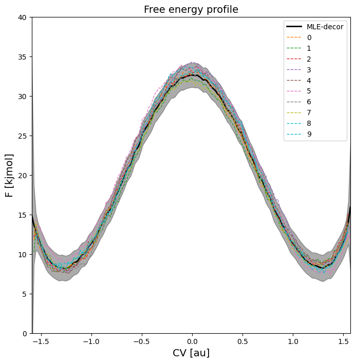
../_images/tut_advanced_error_estimation_51_1.png

We clearly see that all free energy profiles from the bootstrapped subtrajectories all fall well within the error bar computed by the MLE procedure using the decorrelated data.

Covariance between different points on FEP

It is important to realize that the free energy at $q_1$ is not independent from the free energy at $q_2$ , in other words that the covariance between these points is not negligible. This is not only the case for close neighbors (large positive correlation), but in the present case of a profile with two equistable minima, also between points from these equistable minima (i.e. reactant and product state). The main reason for this the fact that the free energy is derived from a normalized probability and this normalization introduces a strong negative correlation between these two equistable minima, because decreased free energy (i.e. increased probability) for reactant implies increased free energy (i.e. decreased probality) for product.

To illustrate the importance of this, we first plot samples of the full free energy profile according to error bars without covariance (using error_estimate=mle_f) and show the difference with the scenario where we redo the error estimation with explicit covariance using error_estimate=mle_f_cov.

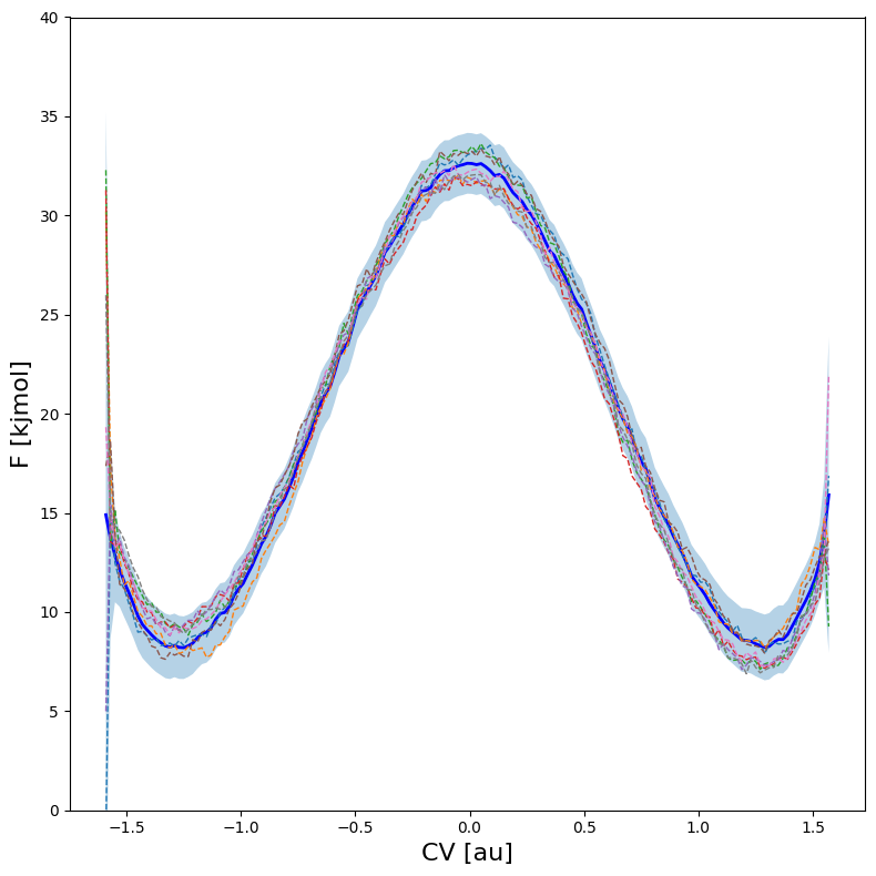
Considering first the free energy profile without covariance, we can plot samples using the plot routine as follows:

[26]:

fep_decor.plot(
    obss      = ['mean']+['sample',]*8,
    linestyles=    ['-']+    ['--',]*8,
    linewidths=      [2]+       [1,]*8,
    colors    =    ['b']+    [None,]*8,
    flims=[0,40]
)

../_images/tut_advanced_error_estimation_55_0.png

As we can see, the error just corresponds to normally random fluctuations on all points individually without any correlation between fluctuations.

We now reconstruct the error on the fep by explicitly taking the covariance into account.

[27]:

hist_cov = Histogram1D.from_wham(bins, trajectories_1, biasses, temp, error_estimate='mle_f_cov', corrtimes=corrtimes, Nscf=10000)
fep_cov = SimpleFreeEnergyProfile.from_histogram(hist_cov, temp, cv_output_unit='au', cv_label='CV', f_output_unit='kjmol')
fep_cov.process_states(lims=[-1.5,-0.2,0.2,1.5])

WARNING: the CV range you specified for the histogram does not cover the entire simulation range in trajectory 127. Simulation samples outside the given CV range were cropped out.
SCF Converged!
---------------------------------------------------------------------
TIMING SUMMARY
  initializing: 00h 00m 00.000s
  histograms  : 00h 00m 00.161s
  bias poten. : 00h 00m 00.008s
  solve scf   : 00h 00m 00.185s
  error est.  : 00h 00m 00.562s
  TOTAL       : 00h 00m 00.919s
---------------------------------------------------------------------
WARNING: multivariate normal sampling failed using Cholesky decomposition, switching to method eigh.
WARNING: multivariate normal sampling failed using Cholesky decomposition, switching to method eigh.
WARNING: multivariate normal sampling failed using Cholesky decomposition, switching to method eigh.
WARNING: multivariate normal sampling failed using Cholesky decomposition, switching to method eigh.
WARNING: multivariate normal sampling failed using Cholesky decomposition, switching to method eigh.

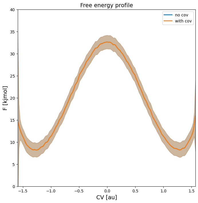
As can be seen in the free energy profile below, the 2-sigma error bar on the entire profile is identical with or without accounting for covariance:

[28]:

plot_profiles([fep_decor,fep_cov], labels=['no cov', 'with cov'], flims=[0,40])

<Figure size 640x480 with 0 Axes>

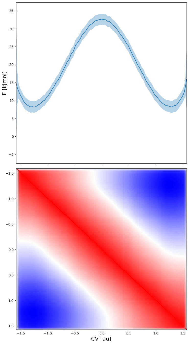
../_images/tut_advanced_error_estimation_59_1.png

However, the coviarance is clearly non neglible as seen in the matrix plot below of the correlation matrix between the various points on the fep. This correlation ranges from 1 (perfect correlation), to 0 (completely uncorrelated) and -1 (perfect anticorrelation).

[29]:

fep_cov.plot_corr_matrix()

<Figure size 640x480 with 0 Axes>

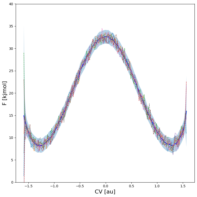
../_images/tut_advanced_error_estimation_61_1.png

Therefore, the error model in fep_cov generates much more reliable ‘samples’ of the full free energy profile by taking into account the full covariance matrix. This can again be plotted using the fep_cov.plot_samples routine:

[30]:

fep_cov.plot(
    obss      = ['mean']+['sample',]*8,
    linestyles=    ['-']+    ['--',]*8,
    linewidths=      [2]+       [1,]*8,
    colors    =    ['b']+    [None,]*8,
    flims=[0,40]
)

WARNING: multivariate normal sampling failed using Cholesky decomposition, switching to method eigh.
WARNING: multivariate normal sampling failed using Cholesky decomposition, switching to method eigh.
WARNING: multivariate normal sampling failed using Cholesky decomposition, switching to method eigh.
WARNING: multivariate normal sampling failed using Cholesky decomposition, switching to method eigh.
WARNING: multivariate normal sampling failed using Cholesky decomposition, switching to method eigh.
WARNING: multivariate normal sampling failed using Cholesky decomposition, switching to method eigh.
WARNING: multivariate normal sampling failed using Cholesky decomposition, switching to method eigh.
WARNING: multivariate normal sampling failed using Cholesky decomposition, switching to method eigh.

../_images/tut_advanced_error_estimation_63_1.png

This figure clearly illustrates that higher free energy for reactant state also implies lower free energy for the product state and vice versa!

Error propagation

Such correlated estimates of samples of the full free energy profile allows to do proper error propagation, i.e. to compute the free energy of integrated macrostates. To illustrate that, we compute propagate the error on the profile to that on the microstate/macrostate free energy derived from the profile for both the fep without covariance (i.e. fep_decor) and that with covariance estimate (i.e. fep_cov):

[31]:

fep_decor.process_states(lims=[-1.5,-0.5,0.5,1.5], verbose=True)

MICROSTATE ts:
--------------
  index =  None
  F     = 33.706 +- 0.803 kjmol
  CV    = -0.003 +- 0.144 au

MICROSTATE r:
--------------
  index =  None
  F     = 7.155 +- 0.995 kjmol
  CV    = -1.284 +- 0.118 au

MICROSTATE p:
--------------
  index =  None
  F     = 7.087 +- 1.023 kjmol
  CV    = 1.278 +- 0.110 au

MACROSTATE R:
--------------
  F       = 10.330 +- 0.346 kjmol
  CV Mean = -1.238 +- 0.015 au
  CV StD  = 0.144 +- 0.009 au

MACROSTATE P:
--------------
  F       = 10.423 +- 0.311 kjmol
  CV Mean = 1.233 +- 0.019 au
  CV StD  = 0.145 +- 0.009 au

[32]:

fep_decor.plot(flims=[0,35])

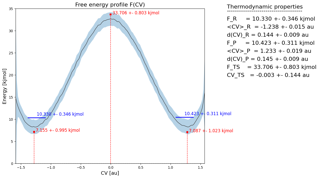
../_images/tut_advanced_error_estimation_68_0.png

Here, we clearly see that estimate of the red microstate dots representing local minima (reactant ant product) and maxima (transition state) are located on the lower/upper edge of the error bar respectively. That is because in the random samples of the full fep, the lack of correlation between neighboring points (which results in uncorrelated fluctuation on the free energy of each point) ensures that there will always be a point close to the lower/upper error bar boundary. Furthermore, we also see a much lower error on the blue macrostates representing the integral over reactant (left of ts) and product (right of ts) microstates. This is because the random fluctuation resulting the uncorrelated error bar is moslty filtered out by the integral.

This clearly indicates the failure of uncorrelated error bars for propagation towards derived properties. Instead, we need to do such error propagation using correlated error bars coming from accounting for the full covariance matrix.

[33]:

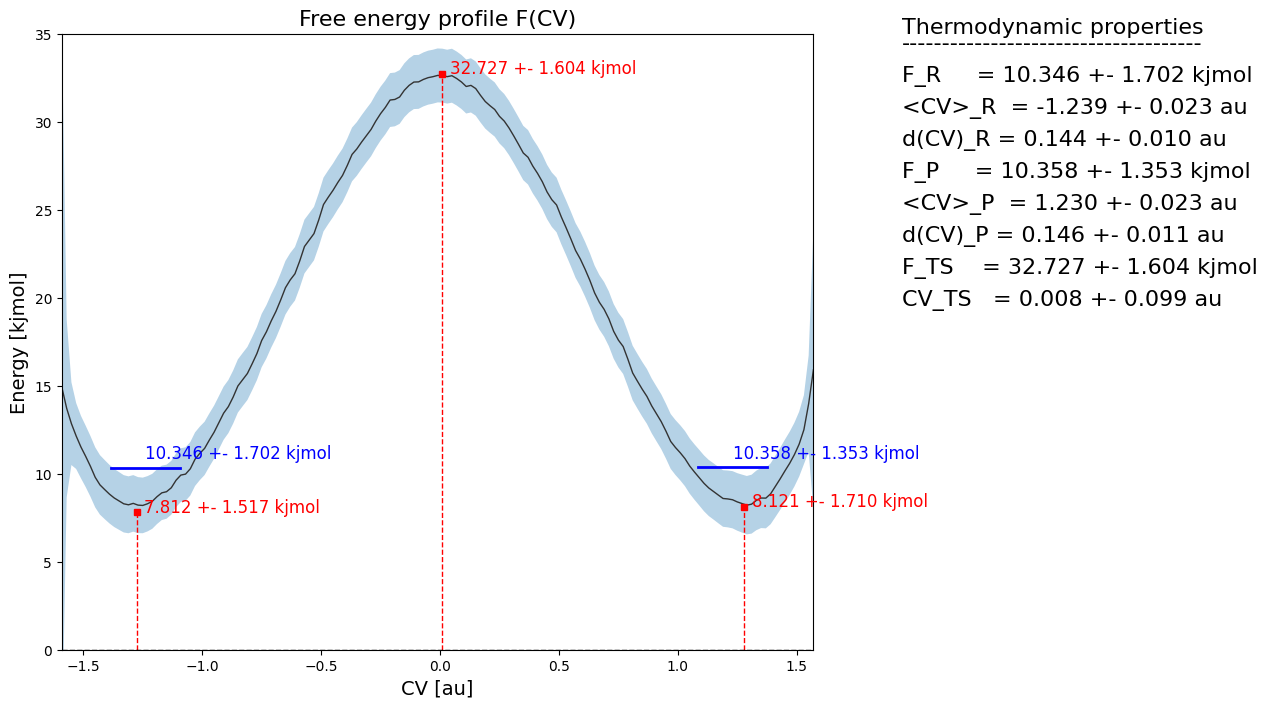
fep_cov.process_states(lims=[-1.5,-0.5,0.5,1.5], verbose=True)

WARNING: multivariate normal sampling failed using Cholesky decomposition, switching to method eigh.
MICROSTATE ts:
--------------
  index =  None
  F     = 32.727 +- 1.604 kjmol
  CV    = 0.008 +- 0.099 au

WARNING: multivariate normal sampling failed using Cholesky decomposition, switching to method eigh.
MICROSTATE r:
--------------
  index =  None
  F     = 7.812 +- 1.517 kjmol
  CV    = -1.275 +- 0.095 au

WARNING: multivariate normal sampling failed using Cholesky decomposition, switching to method eigh.
MICROSTATE p:
--------------
  index =  None
  F     = 8.121 +- 1.710 kjmol
  CV    = 1.279 +- 0.068 au

WARNING: multivariate normal sampling failed using Cholesky decomposition, switching to method eigh.
MACROSTATE R:
--------------
  F       = 10.346 +- 1.702 kjmol
  CV Mean = -1.239 +- 0.023 au
  CV StD  = 0.144 +- 0.010 au

WARNING: multivariate normal sampling failed using Cholesky decomposition, switching to method eigh.
MACROSTATE P:
--------------
  F       = 10.358 +- 1.353 kjmol
  CV Mean = 1.230 +- 0.023 au
  CV StD  = 0.146 +- 0.011 au

[34]:

fep_cov.plot(flims=[0,35])

../_images/tut_advanced_error_estimation_71_0.png

[ ]: