Extensions – `thermolib.ext`

thermolib.ext.wham1d_bias(int Nsims, int Ngrid, double beta, list biasses, double delta, int bias_subgrid_num, ndarray bin_centers, double threshold=1e-3)

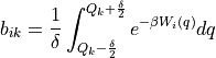
Internal WHAM routine to compute the integrated boltzmann factors of the bias potentials W in each grid interval:

$b_{ik} = \frac{1}{\delta}\int_{Q_k-\frac{\delta}{2}}^{Q_k+\frac{\delta}{2}} e^{-\beta W_i(q)}dq$

This routine implements a conservative algorithm which takes into account that for a given simulation i, only a limited number of grid points $k$ will give rise to a non-zero $b_{ik}$ . This is achieved by first using the bin-center approximation to the integral by computing the factor 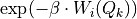$\exp(-\beta\cdot W_i(Q_k))$ on the CV grid (which is faster as there is no integral involved and which is also already a good approximation) and only performing the precise integral when the approximation exceeds the given threshold.

Parameters:

Nsims (int) – the total number of simulations performed
Ngrid (int) – number of points on the CV grid to be used for the histogram.
beta (float) – 1/kT in atomic units with T the temperature at which the simulation was performed
biasses (list of instances of child classes of BiasPotential1D) – list of bias potentials that were applied for each of the simulations.
delta (float) – width of CV-interval ( $\delta$ in equation above) over which the bias is integrated when the bin-center approximation is not sufficient (see doc above)
bias_subgrid_num – the number of grid points used by the wham1d_bias routine for the sub-grid to compute the boltzmann-integrated bias factors in each CV bin. :type bias_subgrid_num: int
bin_center (np.ndarray[double]) – array containing the center of each bin in the histogram for application in the bin-center approximation (see doc above)
threshold – see general documentation above

Returns:

array containing the (integrated) bias on the CV-grid for each simulation, i.e. $b_{ik}$ array from equation above.

Return type:

np.ndarray[double, shape=(Nsims, Ngrid)]

thermolib.ext.wham1d_error(int Nsims, int Ngrid, ndarray Nis, ndarray ps, ndarray fs, ndarray bs, ndarray corrtimes, method='mle_f_cov', p_threshold=0.0, verbosity='off')

Internal WHAM routine that allows to compute the error distribution on the unbiased probability distirbution that is estimated using the WHAM equations. The error estimation is based on the interpretation of the WHAM solutio as a Maximum Likelihood Estimater (MLE), which in term allows to estimate the error based on the Fisher information matrix.

Parameters:

Nsims (int) – the total number of simulations performed
Ngrid (int) – number of points on the CV grid to be used for the histogram.
Nis (np.ndarray[long, shape=(Nsims,)]) – Nis[j] is the number of samples in the trajectory of simulation j
ps (np.ndarray[double, shape=(Ngrid,)]) – the unbiased probability distribution as returned by the wham1d_scf routine. Can contain nan values at specific grid locations (corresponding to disabled bins)
fs (np.ndarray[double, shape=(Nsims,)]) – renormalisation factors fs figuring in the WHAM equations. These are computed as intermediate variables in the wham1d_scf routine. Can contain nan values at specific sim indices (at disabled simulations).
bs (np.ndarray[double, shape=(Nsims,Ngrid)]) – array containing the (integrated) bias on the CV-grid for each simulation, i.e. $b_{ik}$ array from equation above.
corrtimes (np.ndarray[double, shape=(Nsims,)]) – array of (integrated) correlation times of the CV, one for each simulation. Such correlation times will be taken into account during the error estimation and hence make it more reliable. If set to None, the CV trajectories will be assumed to contain fully uncorrelated samples (which is not true when using trajectories representing each subsequent step from a molecular dynamics simulation). More information can be found in the user guide. This input can be generated using the decorrelate routine.
method (str or None, optional, default='mle_f_cov') –
specification of the method on how to perform the estimation of the error distribution. One of following options is available:
- mle_p - Estimating the error directly for the probability of each bin in the histogram. This method does not explicitly impose the positivity of the probability.
- mle_p_cov - Estimate the full covariance matrix for the probability of all bins in the histogram. In other words, appart from the error on the probability/free energy of a bin itself, we now also account for the covariance between the probabilty/free energy of the bins. This method does not explicitly impose the positivity of the probability.
- mle_f - Estimating the error for minus the logarithm of the probability, which is proportional to the free energy (hence f in mle_f). As the probability is expressed as $\propto e^{-f}$ , its positivity is explicitly accounted for.
- mle_f_cov - Estimate the full covariance matrix for minus the logarithm of the probability of all bins in the histogram. In other words, appart from the error on the probabilty/free energy of a bin itself (including explicit positivity constraint), we now also account for the covariance between the probability/free energy of the bins.
p_threshold (float, optional, default=0.0) – only relevant when error estimation is enabled (see parameter error_estimate). When error_p_threshold is set to x, bins in the histogram for which the probability resulting from the trajectory is smaller than x will be disabled for error estimation (i.e. its error will be set to np.nan). It is mainly usefull in the case of 2D histograms,as illustrated in one of the tutorial notebooks.
verbosity (str, optional, default='off') – specify the level of verbosity of the current routine

Returns:

the distribution of the error on the unbiased probability distribution

Return type:

GaussianDistribution (if method=’mle_p’), MultiGaussianDistribution (if method=’mle_p_cov’), LogGaussianDistribution (if method=’mle_f’), MultiLogGaussianDistribution (if method=’mle_f_cov’)

thermolib.ext.wham1d_hs(int Nsims, int Ngrid, ndarray trajectories, ndarray bins, ndarray Nis)

Internal WHAM routine to compute the 1D CV histogram of each (biased) simulation from the given CV trajectories.

Parameters:

Nsims (int) – number of simulations that were done and for which the histogram needs to be constructed
Ngrid (int) – number of points on the CV grid to be used for the histogram.
trajectories (np.ndarray) – array containing the simulation trajectory (i.e. CV samples) for each (biased) simulation
bins (np.ndarray[double, shape=(Ngrid+1,)]) – bin edges for the CV histogram. Should have length one larger than Ngrid
Nis (np.ndarray[long, shape=(Nsims,)]) – Nis[j] is the number of samples in the trajectory of simulation j

Returns Hs:

2 dimensional array containing the CV histograms for each of the (biased) simulations. Hs[i,k] represents the histogram value of the k-th bin for the i-th simulation.

Return type:

np.ndarray[long, shape=(Nsims, Ngrid)]

thermolib.ext.wham1d_scf(ndarray Nis, ndarray Hs, ndarray bs, int Nscf=1000, double convergence=1e-6, double overflow_threshold=1e-150, verbose=False)

Internal WHAM routine to solve the WHAM equations for the unbiased probability distribution

$\frac{1}{f_i} &= \sum_k b_{ik} a_k \\ a_k &= \sum_i \frac{H_{ik}}{\sum_i N_i f_i b_{ik}}$

until self consistency is achieved.

Parameters:

Nis (np.ndarray[long, shape=(Nsims,)]) – Nis[j] is the number of samples in the trajectory of simulation j
Hs (np.ndarray[long, shape=(Nsims, Ngrid)]) – 2 dimensional array containing the CV histograms for each of the (biased) simulations
bs (np.ndarray[double, shape=(Nsims, Ngrid)]) – array containing the (integrated) bias on the CV-grid for each simulation, i.e. $b_{ik}$ array from equation above.
Nscf (int, optional, default=1000) – maximum number of SCF cycles to obtain self-consistency
convergence (double, optional, default=1e-6) – sets criterium determining self-consistency, SCF cycle will stop when the integrated absolute value of the difference between the unbiased probability distribution at the current step and the previous step is smaller then the given convergence parameter.
overflow_threshold (double, optional, default=1e-150) – numerical threshold to avoid overflow errors when calculating the normalization factors and the denominator of the unbiased probability. This determines which simulations and which grid points to ignore. Decreasing it results in a FEP with a larger maximum free energy (lower unbiased probability). If it is too low, imaginary errors arise, so increase if necessary.

Returns:

the unbiased probability distribution on the same grid as all the histograms in the Hs argument.

Return type:

np.ndarray[double, shape=(Ngrid,)]

thermolib.ext.wham2d_bias(int Nsims, int Ngrid1, int Ngrid2, double beta, list biasses, double delta1, double delta2, int bias_subgrid_num1, int bias_subgrid_num2, ndarray bin_centers1, ndarray bin_centers2, double threshold=1e-3)

Compute the integrated boltzmann factors of the biases in each grid interval:

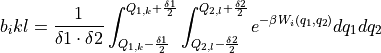
$b_ikl = \frac{1}{\delta1\cdot\delta2}\int_{Q_{1,k}-\frac{\delta1}{2}}^{Q_{1,k}+\frac{\delta1}{2}}\int_{Q_{2,l}-\frac{\delta2}{2}}^{Q_{2,l}+\frac{\delta2}{2}} e^{-\beta W_i(q_1,q_2)}dq_1dq_2$

This routine implements a conservative algorithm which takes into account that for a given simulation i, only a limited number of grid points (k,l) will give rise to a non-zero b_ikl. This is achieved by first using the bin-center approximation to the integral by computing the factor $\exp(-\beta\cdot bias(Q_{1,k},Q_{2,l}))$ on the CV1 and CV2 grid (which is faster as there is no integral involved and which is also already a good approximation for the $b_{ikl}$ array) and only performing the precise integral when the approximation exceeds a threshold.

Parameters:

Nsims (int) – the total number of simulations performed
Ngrid1 (int) – number of points on the CV1 grid to be used for the histogram.
Ngrid2 (int) – number of points on the CV2 grid to be used for the histogram.
beta (float) – 1/kT in atomic units with T the temperature at which the simulation was performed
biasses (list of instances of child classes of BiasPotential1D) – list of bias potentials that were applied for each of the simulations.
delta1 (float) – width of CV1-interval ( $\delta_1$ in equation above) over which the bias is integrated when the bin-center approximation is not sufficient (see doc above)
delta2 (float) – width of CV2-interval ( $\delta_2$ in equation above) over which the bias is integrated when the bin-center approximation is not sufficient (see doc above)
bias_subgrid_num1 – the number of grid points along CV1 used by the wham2d_bias routine for the sub-grid to compute the boltzmann-integrated bias factors in each (CV1,CV2) bin. :type bias_subgrid_num: int
bias_subgrid_num2 – the number of grid points along CV2 used by the wham2d_bias routine for the sub-grid to compute the boltzmann-integrated bias factors in each (CV1,CV2) bin. :type bias_subgrid_num2: int
bin_centers1 (np.ndarray[double]) – array containing the center (in CV1 direction) of each bin in the histogram for application in the bin-center approximation (see doc above)
bin_centers2 (np.ndarray[double]) – array containing the center (in CV2 direction) of each bin in the histogram for application in the bin-center approximation (see doc above)
threshold – see general documentation above

Returns:

array containing the (integrated) bias on the CV-grid for each simulation, i.e. $b_{ik}$ array from equation above. bs[i,k,l] represents the bias value of bin (k,l) in (CV1,CV2)-space for the i-th simulation.

Return type:

np.ndarray[double, shape=(Nsims,Ngrid1,Ngrid2)]

thermolib.ext.wham2d_error(ndarray ps, ndarray fs, ndarray bs, ndarray Nis, ndarray corrtimes, method='mle_f', p_threshold=0.0, verbosity='off')

Internal WHAM routine that allows to compute the error distribution on the unbiased probability distirbution that is estimated using the WHAM equations. The error estimation is based on the interpretation of the WHAM solutio as a Maximum Likelihood Estimater (MLE), which in term allows to estimate the error based on the Fisher information matrix.

Parameters:

ps (np.ndarray[double, shape=(Ngrid1, Ngrid2)]) – the unbiased probability density as returned by the wham2d_scf routine. Can contain nan values at specific grid locations (corresponding to disabled bins)
fs (np.ndarray[double, shape=(Nsims,)]) – renormalisation factors fs figuring in the WHAM equations. These are computed as intermediate variables in the wham2d_scf routine. Can contain nan values at specific sim indices (at disabled simulations).
bs (np.ndarray[double, shape=(Nsim,Ngrid1,Ngrid2)]) – the biasses (for each simulation) precomputed on the 2D CV grid
Nis (np.ndarray[long, shape=(Nsim,)]) – the number of simulation steps in each simulation
corrtimes (np.ndarray[double, shape=(Nsims,)]) – array of (integrated) correlation times of the CV, one for each simulation. Such correlation times will be taken into account during the error estimation and hence make it more reliable. If set to None, the CV trajectories will be assumed to contain fully uncorrelated samples (which is not true when using trajectories representing each subsequent step from a molecular dynamics simulation). More information can be found in the user guide. This input can be generated using the decorrelate routine.
method –
specification of the method on how to perform the estimation of the error distribution. One of following options is available:
- mle_p - Estimating the error directly for the probability of each bin in the histogram. This method does not explicitly impose the positivity of the probability.
- mle_p_cov - Estimate the full covariance matrix for the probability of all bins in the histogram. In other words, appart from the error on the probability/free energy of a bin itself, we now also account for the covariance between the probabilty/free energy of the bins. This method does not explicitly impose the positivity of the probability.
- mle_f - Estimating the error for minus the logarithm of the probability, which is proportional to the free energy (hence f in mle_f). As the probability is expressed as $\propto e^{-f}$ , its positivity is explicitly accounted for.
- mle_f_cov - Estimate the full covariance matrix for minus the logarithm of the probability of all bins in the histogram. In other words, appart from the error on the probabilty/free energy of a bin itself (including explicit positivity constraint), we now also account for the covariance between the probability/free energy of the bins.
p_threshold (float, optional, default=0.0) – only relevant when error estimation is enabled (see parameter error_estimate). When error_p_threshold is set to x, bins in the histogram for which the probability resulting from the trajectory is smaller than x will be disabled for error estimation (i.e. its error will be set to np.nan). It is mainly usefull in the case of 2D histograms,as illustrated in one of the tutorial notebooks.
verbosity (str, optional, default='off') – specify the level of verbosity of the current routine

Returns:

the distribution of the error on the unbiased probability distribution

Return type:

GaussianDistribution (if method=’mle_p’), MultiGaussianDistribution (if method=’mle_p_cov’), LogGaussianDistribution (if method=’mle_f’), MultiLogGaussianDistribution (if method=’mle_f_cov’)

thermolib.ext.wham2d_hs(int Nsims, int Ngrid1, int Ngrid2, ndarray trajectories, ndarray bins1, ndarray bins2, ndarray Nis)

Internal WHAM routine to compute the 2D CV histogram of each (biased) simulation from the given CV trajectories.

Parameters:

Nsims (int) – number of simulations that were done and for which the histogram needs to be constructed
Ngrid1 (int) – number of points on the CV1 grid to be used for the histogram.
Ngrid2 (int) – number of points on the CV2 grid to be used for the histogram.
trajectories (np.ndarray) – array containing the simulation trajectory (i.e. [CV1,CV2] samples) for each (biased) simulation
bins1 (np.ndarray[double]) – bin edges for CV1 in the histogram. Should have length one larger than Ngrid1
bins2 (np.ndarray[double]) – bin edges for CV2 in the histogram. Should have length one larger than Ngrid2
Nis (np.ndarray[long]) – Nis[j] is the number of samples in the trajectory of simulation j

Returns Hs:

3 dimensional array containing the (CV1,CV2) histograms for each of the (biased) simulations. Hs[i,k,l] represents the histogram value of bin (k,l) in (CV1,CV2)-space for the i-th simulation.

Return type:

np.ndarray[long, ndim=3]

thermolib.ext.wham2d_scf(ndarray Nis, ndarray Hs, ndarray bs, ndarray pinit, int Nscf=1000, double convergence=1e-6, double overflow_threshold=1e-150, verbose=False)

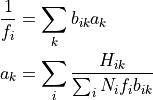
Internal WHAM routine to solve the 2D WHAM equations which can, after flattening the 2D unbiased probability histogram $a_{kl}$ to a 1D array $a_{k}$ , be written as

$\frac{1}{f_i} &= \sum_k b_{ik} a_k \\ a_k &= \sum_i \frac{H_{ik}}{\sum_i N_i f_i b_{ik}}$

which clearly requires an iterative solution. To avoid floating point errors in the calculation of the first equation, we check whether f_i > overflow_threshold. Similarly, we check whether the denominator of equation 2 > overflow_threshold. This corresponds to only keeping those simulations with relevant information.

Parameters:

Nis (np.ndarray[double, shape=(Nsims, Ngrid1, Ngrid2)]) – the number of simulation steps in each simulation
Hs – the histogram counts for each simulation, for each grid point
bs (np.ndarray[double, shape=(Nsims, Ngrid1, Ngrid2)]) – the biasses (for each simulation) precomputed on the 2D CV grid
pinit (np.ndarray[double, shape=(Ngrid1, Ngrid2)]) – the initial unbiased probability density
Nscf (int, optional, default=1000) – maximum number of scf cycles, convergence should be reached before Nscf steps
convergence (double, optional, default=1e-6) – convergence criterion for scf cycle, if integrated difference (sum of the absolute element-wise difference between subsequent predictions of the unbiased probability a_k) is lower than this value, SCF is converged
overflow_threshold (double, optional, default=1e-150) – numerical threshold to avoid overflow errors when calculating the normalization factors and the denominator of the unbiased probability a_k. This determines which simulations and which grid points to ignore. Decreasing it results in a FES with a larger maximum free energy (lower unbiased probability). If it is too low, imaginary errors (sigma^2) arise, so increase if necessary.

Returns:

the unbiased probability distribution on the same grid as all the histograms in the Hs argument.

Return type:

np.ndarray[double, shape=(Ngrid1,Ngrid2)]

Extensions – thermolib.ext

Extensions – `thermolib.ext`