Computing the reaction rate

To compute the reaction rate according to transition state theory, we need to apply the following formula:

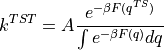
$k^{TST} &= A \frac{e^{-\beta F(q^{TS})}}{\int e^{-\beta F(q)}dq}$

with:

$A &= \sqrt{\frac{1}{2\pi\beta}}\left\langle \left|\vec{\nabla}_x Q\right| \right\rangle_{TS}$

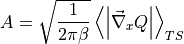
As we can see, the free energy profile $F(q)$ is figuring in this expression, which we already discussed in detail in this user guide. However, in order to compute $k^{TST}$ , we also need the prefactor $A$ which represents the TS-constrained ensemble average of the norm of the mass-weighted gradient of the collective variable, which is information not present in the free energy profile. However, we can extract it from the simulation trajectories of the original simulation, more specifically those trajectories that sample the transition state. In order to extract the required prefactor using ThermoLIB, we first need to define the collective variable mathematically so that we can compute its gradient. This is done using the available classes in the CV module.

To illustrate the definition of the CV, we consider an example in which the CV is given by a linear combination of so-called coordination numbers

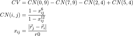
$CV &= CN(0,9) - CN(7,9) - CN(2,4) + CN(5,4) \\ CN(i,j) &= \frac{1-x_{ij}^6}{1-x_{ij}^{12}} \\ x_{ij} &= \frac{\left|\vec{r}_j-\vec{r}_i\right|}{r0}$

Here, CN(i,j) represents the coordination number (roughly the number of chemical bonds) between atoms with indices i and j. r0 is a reference for the length of a typical bond and will in our example be set to r0=1.4*angstrom. The above CV can be defined in thermolib using the CoordinationNumber and LinearCombination classes as follows:

from thermolib.thermodynamics.cv import CoordinationNumber, LinearCombination
C1 = CoordinationNumber([[0,9]], r0=1.4*angstrom)
C2 = CoordinationNumber([[7,9]], r0=1.4*angstrom)
C3 = CoordinationNumber([[2,4]], r0=1.4*angstrom)
C4 = CoordinationNumber([[5,4]], r0=1.4*angstrom)
CV = LinearCombination([C1,C2,C3,C4], [1., -1., -1., 1.])

To extract the prefactor A, we first need to know which simulation trajectories contain relevant samples in the transition state region. Assume that we have access to the XYZ trajectory files of each simulation (we need all coordinates of all atoms if we want to compute the gradient of the collective variable) in the form of uXX.xyz files with XX indicating the XX-th simulation trajectory. We first make an educated guess of which trajectories have transition state samples, e.g. trajectories 61 to 68, and verify this guess by simply plotting the corresponding histograms (using the techniques documented in this user guide):

fns = ['u%i.xyz' for i in range(61,68)]
hists = []
bins = np.arange(-0.15, 0.15, 0.001)
cv_comp = CVComputer([CV])
for fn in fns:
    cv_data = cv_comp(fn)
    hist = Histogram1D.from_single_trajectory(cv_data, bins)
    hists.append(hist)
plot_histograms(hists, labels=fns)

Such code generates a plot as given below:

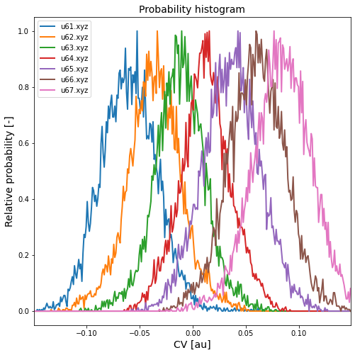
This plot clearly shows us that for example trajectory u64.xyz contains many relevant samples (TS around cv=0.00). We could also proceed using multiple trajectories, e.g. u63.xyz and u64.xyz, but that will prevent us from doing block averaging to estimate the error on the prefactor later on. We initialize an instance of the RateFactorEquilibrium class for extracting the rate prefactor for an equilibrium simulation (eg. umbrella around TS). As mentioned before, the ensemble average for the A prefactor is a constrained average in which the system is constrained to be in the transition state. Obviously, we cannot define the transition state as having a CV of precisly 0.000, instead we need to assign it an interval with a non-zero width. This interval is denoted as CV_TS_lims below. From the histograms above, we choose this interval as [-0.01,0.01]. As such, we can compute the rate prefactor (and its error using block averaging or blav) as follows:

from thermolib.kinetics.rate import RateFactorEquilibrium
rate = RateFactorEquilibrium(CV, [-0.01, 0.01], temp)
rate.process_trajectory('u64.xyz')
A, A_dist = rate.result_blav(plot=True, fitrange=[1,300])

The block averaging routine produces the following output and plot:

Rate factor with block averaging:
---------------------------------
  A = 17.461 +- 0.012 1e12*au/s (3215 TS samples, int. autocorr. time = 1.000 timesteps)

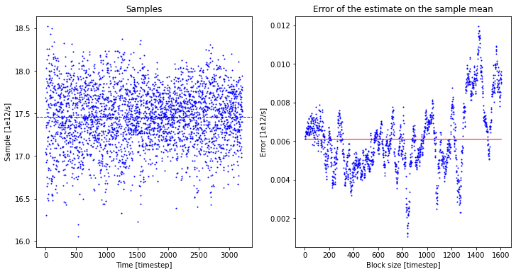
In this particular case, all TS samples of $\left|\vec{\nabla}_x Q\right|$ figuring in the expression for A seem to be uncorrelated (as indicated by an integrated correlation time of 1) and hence result in a very small error. This is not necessarily always the case. Finally, we can compute the reaction rate (including his error) from the free energy profile (and its error) and the prefactor A (and its error):

#setting verbose to True will print the results in a formatted fashion
rate_results = rate.compute_rate(fep, verbose=True)

Finally, if you now parse the rate instance to the plotting routine of the fep instance, it will include the reaction rates as well as the related phenomenological free energy barriers in the plot:

fep.plot(rate=rate)

which produces a plot such as:

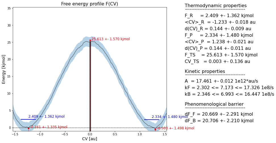
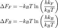
Herein, kF/kB represent the rate of the forward/backward reaction, while dF_F/dF_B represent the corresponding phenomenological free energy barriers that are defined as:

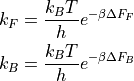
$k_F &= \frac{k_BT}{h}e^{-\beta \Delta F_F} \\ k_B &= \frac{k_BT}{h}e^{-\beta \Delta F_B}$

or:

$\Delta F_F &= -k_BT\ln\left(\frac{h k_F}{k_B T}\right) \\ \Delta F_B &= -k_BT\ln\left(\frac{h k_B}{k_B T}\right)$