Tutorial 8 - Transformation of 2D free energy surfaces

Introduction

This notebook illustrates the usage of ThermoLIB to transform a 2D free energy surface in terms of collective variables (CV1,CV2) towards a new FES in terms of new collective variables (Q1,Q2) in which the relation between (CV1,CV2) and (Q1,Q2) is given as a deterministic transformation formula. For the purpose of this illustration, we will chose a transformation that encodes a simply rotation in the (CV1,CV2) plane. Furthermore, to validate the implementation, we will also project the original FES on the CV1 axis and compare with the projection of the rotated FES on the rotated CV1 axis.

[5]:

%load_ext autoreload
%autoreload 2

The autoreload extension is already loaded. To reload it, use:
  %reload_ext autoreload

[6]:

from thermolib.thermodynamics.fep import FreeEnergySurface2D, SimpleFreeEnergyProfile, plot_profiles
from thermolib.thermodynamics.histogram import Histogram2D
from thermolib.tools import read_wham_input, decorrelate
from thermolib.thermodynamics.trajectory import ColVarReader
from thermolib.error import Propagator
from thermolib.units import *

import numpy as np, matplotlib.pyplot as pp, time

Define some file/path variables

[7]:

fn_meta = '/home/lvduyfhu/hpc/data_vo/shared/massimo/for_Louis/H-ZSM-5_ethylation/wham_input_2D.txt' #location of the plumed metadata file containing all information of the umbrella sampling

Construction of original 2D FES

[8]:

colvar_reader = ColVarReader([1,2], units=['au','au'])
temp, biasses, trajectories = read_wham_input(
    fn_meta, colvar_reader, 'colvars/colvar_%s.dat',
    bias_potential='Parabola2D', q01_unit='au', q02_unit='au', kappa1_unit='kjmol', kappa2_unit='kjmol',
)

[9]:

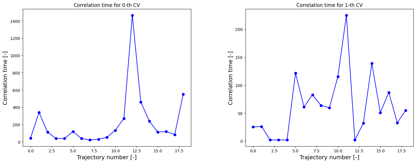
corrtimes = decorrelate(trajectories, plot=True)

/home/lvduyfhu/miniconda3/envs/test/lib/python3.14/site-packages/thermolib/tools.py:960: OptimizeWarning: Covariance of the parameters could not be estimated
  pars, pcovs = curve_fit(function, upper_envelope_indices, upper_envelope_values, **curve_fit_kwargs)

<Figure size 640x480 with 0 Axes>

../_images/tut_advanced_transformations_2D_9_2.png

Next, we construct the 2D probability histogram on the given 2D CV grid (defined by bins) using the WHAM routine.

[10]:

bins = [np.arange(1,4.025,0.025), np.arange(-2.5,0.025,0.025)]
hist = Histogram2D.from_wham(bins, trajectories, biasses, temp, error_estimate='mle_f_cov', corrtimes=corrtimes, error_p_threshold=1e-4)
hist_noerror = Histogram2D.from_wham(bins, trajectories, biasses, temp)

WARNING: could not converge WHAM equations to convergence of 1.000e-06 in 1000 steps!
  SCF did not converge!

---------------------------------------------------------------------
TIMING SUMMARY
  initializing: 00h 00m 00.000s
  histograms  : 00h 00m 00.022s
  bias poten. : 00h 00m 00.730s
  solve scf   : 00h 00m 00.345s
  error est.  : 00h 00m 13.492s
  TOTAL       : 00h 00m 14.592s
---------------------------------------------------------------------
WARNING: could not converge WHAM equations to convergence of 1.000e-06 in 1000 steps!
  SCF did not converge!

---------------------------------------------------------------------
TIMING SUMMARY
  initializing: 00h 00m 00.000s
  histograms  : 00h 00m 00.017s
  bias poten. : 00h 00m 00.765s
  solve scf   : 00h 00m 00.317s
  error est.  : 00h 00m 00.000s
  TOTAL       : 00h 00m 01.100s
---------------------------------------------------------------------

[11]:

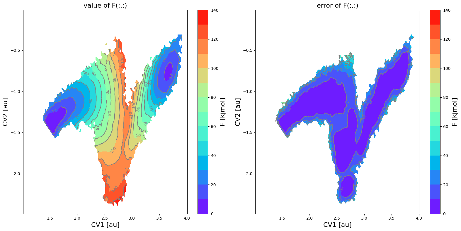
fes = FreeEnergySurface2D.from_histogram(hist, temp)
fes_noerror = FreeEnergySurface2D.from_histogram(hist_noerror, temp)
fes.set_ref(ref='min')
fes_noerror.set_ref(ref='min')
fes.plot(obss=['value', 'error'], cmap='rainbow', flims=[0,140], ncolors=14)

<Figure size 640x480 with 0 Axes>

../_images/tut_advanced_transformations_2D_12_1.png

[12]:

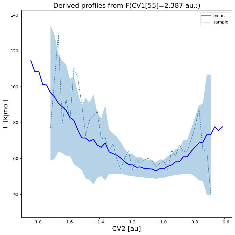
fes.plot(slicer=[55,slice(None)], obss=['mean', 'sample'], linewidths=[2,1], linestyles=['-', '--'], colors=['b',None])

WARNING: multivariate normal sampling failed using Cholesky decomposition, switching to method eigh.

../_images/tut_advanced_transformations_2D_13_1.png

Transformation to new CVs

We transform $F_\text{CV}(CV_1,CV_2)$ to $F_\text{Q}(Q_1,Q_2)$ with:

:nbsphinx-math:`begin{align}: Q_1 &= frac{sqrt{2}}{2}left(CV_1 - 2.75 + CV_2 + 1.25right) \ Q_2 &= frac{sqrt{2}}{2}left(CV_2 + 1.25 - CV_1 + 2.75right)

end{align}`

which simply encodes a rotation over 45 degrees around the point $(CV_1,CV_2)=(2.27,-1.25)$

[13]:

f1 = lambda x,y: np.sqrt(2)/2*(x-2.75+y+1.25)
f2 = lambda x,y: np.sqrt(2)/2*(y+1.25-x+2.75)
derivatives = lambda x,y: ((np.sqrt(2)/2, np.sqrt(2)/2), (-np.sqrt(2)/2, np.sqrt(2)/2))
q1s = np.arange(-1.2,1.4+0.025,0.025)
q2s = np.arange(-1.0,1.0+0.025,0.025)
fes2 = fes.transform_function((f1,f2), q1s, q2s, derivatives=derivatives, cv1_label='Q1', cv2_label='Q2')

WARNING: multivariate normal sampling failed using Cholesky decomposition, switching to method eigh.

[14]:

fes2.plot(obss=['value', 'error'], cmap='rainbow', flims=[0,140], ncolors=14)

<Figure size 640x480 with 0 Axes>

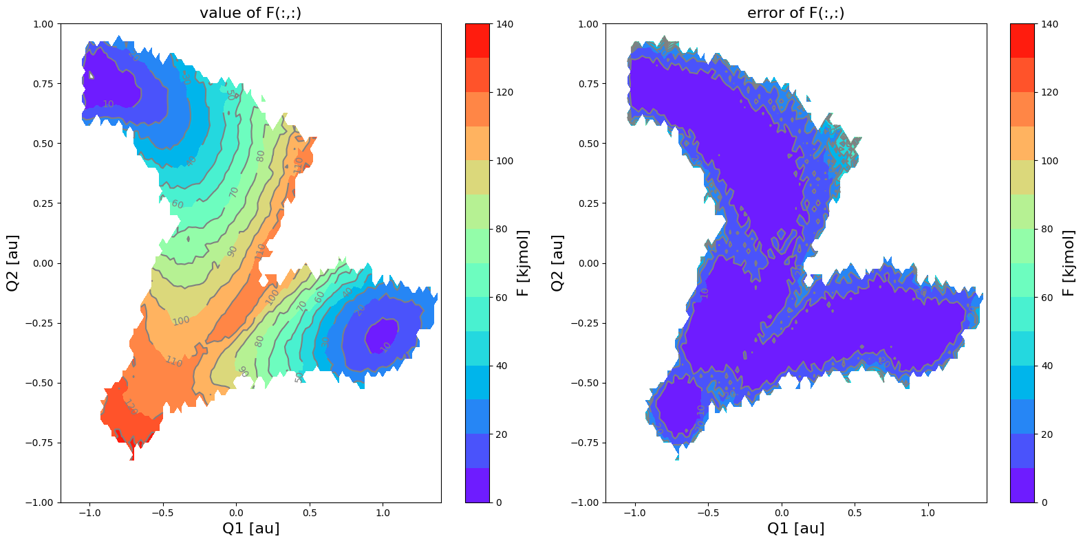
../_images/tut_advanced_transformations_2D_17_1.png

Both the free energy itself as well as its error bar indeed seem to represent a rotated version of the original.

Projection comparison

As a further comparison, we project the original FES on CV1 as well as the new FES on $f(Q_1,Q_2)=\frac{\sqrt{2}}{2}\left(Q_1-Q_2\right)+2.75=CV_1$ and compare on a 1D plot (with error bar).

[15]:

fep = fes.project_cv1()

WARNING: multivariate normal sampling failed using Cholesky decomposition, switching to method eigh.

[16]:

fun = lambda x,y: np.sqrt(2)/2*(x-y)+2.75
cv1s = np.arange(1,4.025,0.025)
fep2 = fes2.project_function(fun, cv1s)

WARNING: multivariate normal sampling failed using Cholesky decomposition, switching to method eigh.

[17]:

plot_profiles([fep,fep2], labels=['before trans','after trans'], linestyles=['-','--'], colors=['b','k'], flims=[-40,140])

<Figure size 640x480 with 0 Axes>

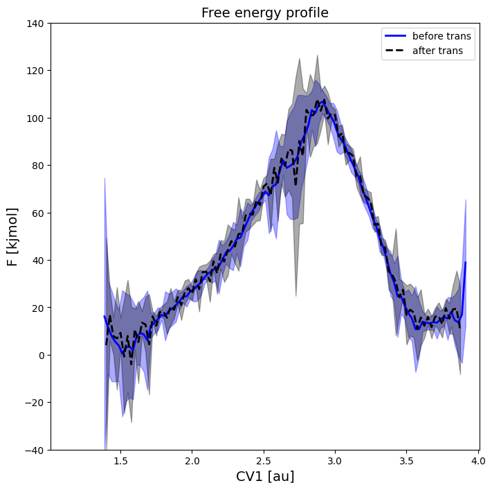
../_images/tut_advanced_transformations_2D_23_1.png

This plot clearly illustrates that both projections are the same, further validating the implementation.