Skip to content

Learning algorithms

The endgame of psiflow is to allow for the seamless development and scalable execution of online learning algorithms for interatomic potentials. The BaseLearning class provides an interface based on which such algorithms can be implemented, and it has the following characteristics:

  • learning.run(): performs the actual active learning using a BaseModel, a BaseReference, and a list of BaseWalker instances. Optionally, you can also specify an initial dataset which can be used to bootstrap the learning (see below).
  • an output folder: used for storing intermediate models, (labeled) datasets, walkers, and reported metrics.
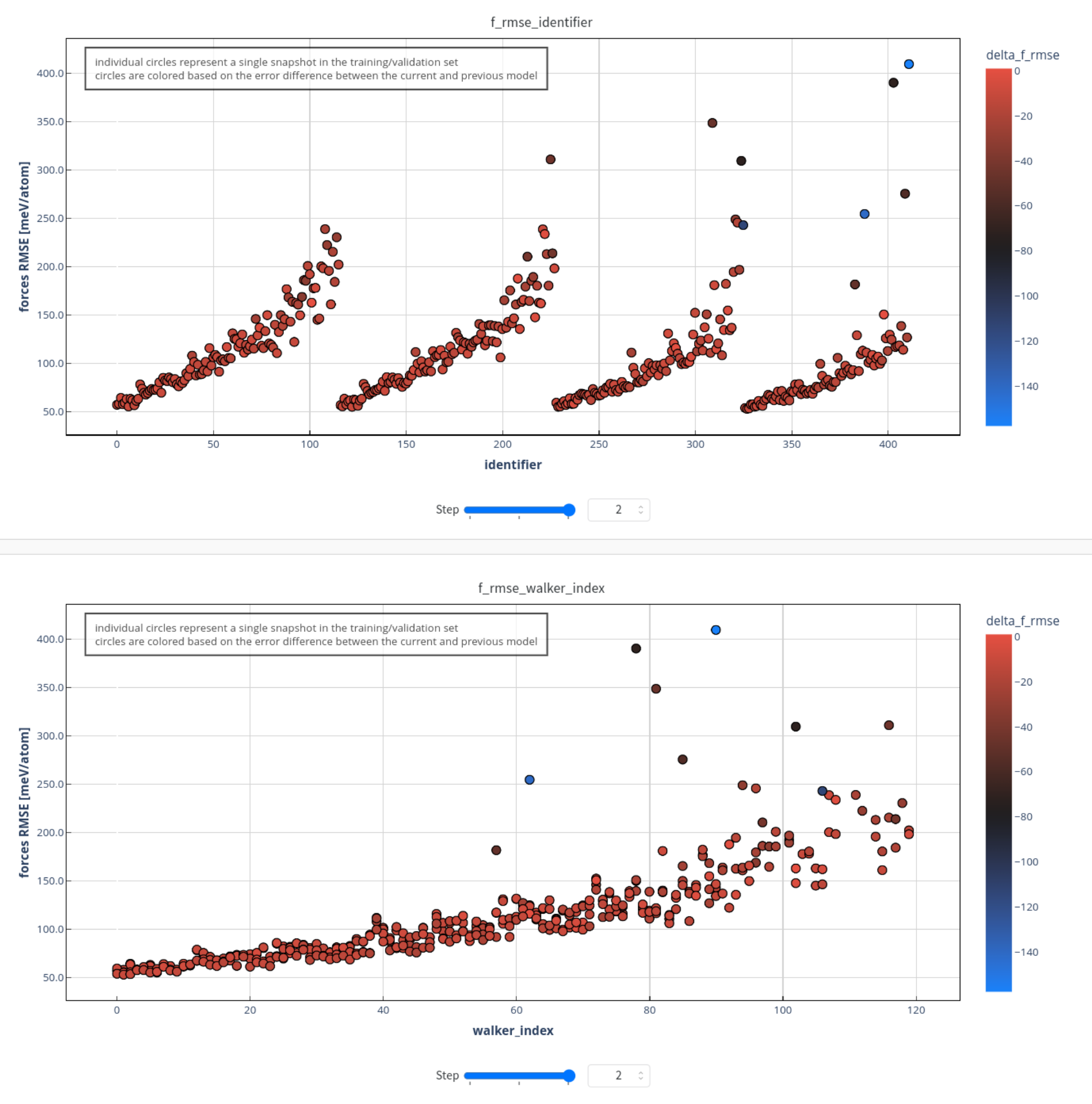
  • state identifier: to facilitate logging and/or debugging of the active learning progress, each successfully labeled state is immediately given a unique identifier (an integer). This is necessary in order to keep track of which molecular dynamics log or DFT evaluation log belongs to which state, especially when data is shuffled in each iteration. The identifier is stored in the info dict of each of the FlowAtoms instances, and is therefore also human-readable in the dataset XYZ files.
  • metrics: the Metrics helper class is used to compute and save various error metrics and other relevant diagnostics during online learning. Examples are per-element validation RMSEs or collective variables of the sampled data:
    dataset.log
    +------------+--------+--------+-------+----------+----------+----------+----------+-----------+
    | identifier | e_rmse | f_rmse |    CV | f_rmse_H | f_rmse_C | f_rmse_N | f_rmse_I | f_rmse_Pb |
    +------------+--------+--------+-------+----------+----------+----------+----------+-----------+
    |          0 |   0.23 |  32.15 | -4.54 |    23.82 |    47.04 |    37.72 |    27.97 |     46.47 |
    |          1 |   0.27 |  31.72 | -4.45 |    23.13 |    43.52 |    34.12 |    28.43 |     52.42 |
    |          2 |   0.45 |  33.60 | -4.49 |    27.02 |    44.40 |    40.34 |    27.77 |     48.51 |
    |          3 |   0.39 |  33.02 | -4.44 |    26.52 |    50.11 |    36.97 |    27.50 |     45.21 |
    |          4 |   0.36 |  31.75 | -4.47 |    25.15 |    41.36 |    37.35 |    27.10 |     47.16 |
    |          5 |   0.35 |  34.00 | -4.41 |    28.04 |    43.99 |    39.52 |    28.56 |     49.31 |
    ...
    
    or the (a posteriori) error of individual walkers and other relevant information:
    walkers.log
    +--------------+---------+----------+--------+--------------+-------------+------------+-------+--------+-------------------------------------+
    | walker_index | counter | is_reset | f_rmse | disagreement | temperature | identifier |    CV | e_rmse |                              stdout |
    +--------------+---------+----------+--------+--------------+-------------+------------+-------+--------+-------------------------------------+
    |            0 |    1000 |    False |  47.33 |         None |      135.79 |        150 | -4.61 |   4.04 | task_7028_molecular_dynamics_openmm |
    |            1 |    1000 |    False |  50.69 |         None |      142.89 |        151 | -4.39 |   4.11 | task_7046_molecular_dynamics_openmm |
    |            2 |    1000 |    False |  46.34 |         None |      140.72 |        152 | -4.61 |   4.07 | task_7064_molecular_dynamics_openmm |
    |            3 |    1000 |    False |  43.71 |         None |      136.12 |        153 | -4.45 |   4.24 | task_7082_molecular_dynamics_openmm |
    ...
    
    Although optional, it also provides a convenient Weights & Biases interface for easier navigation and interpretation of all of the metrics.
  • (optional) pretraining: pretraining is used to bootstrap active learning runs. In essence, it makes the model familiar with the chemical bonds in the system and ensures that it doesn't go too crazy during sampling in the first few iterations. During pretraining, a minimal set of configurations is generated by applying random perturbations to the atomic positions and/or unit cell vectors (typically about 0.05 A in magnitude). These configurations are then evaluated using the provided BaseReference instance after which the obtained data is split into training and validation in order to pretrain the model. When learning.run() is called, it decides whether or not to perform pretraining based on whether the model has already been initialized as well as whether initial data is presented (i.e. there are four possible scenarios):
    • initialized model, initial data: start with active learning and append generated data to the initial data;
    • uninitialized model, initial data: train the model on the initial data before starting the active learning;
    • uninitialized model, no initial data: execute pretraining using the atomic geometries stored in the walkers. The size of the pretraining dataset as well as the magnitude of the perturbations is specified as keyword arguments to the learning algorithm;
    • initialized model, no initial data: initialize an empty dataset and start with active learning.

The following keyword arguments are shared between all BaseLearning subclasses

  • path_output : pathlib.Path | str : defines the output directory in which all results are stored
  • train_valid_split : float = 0.9 : determines the fraction of all data that is used for training (typically 0.9)
  • pretraining_nstates : int = 50 : size of the pretraining dataset
  • pretraining_amplitude_pos : float = 0.05 : amplitude of the perturbations (in Angstrom) that is applied on the positions in order to generate the pretraining dataset
  • pretraining_amplitude_box : float = 0.05 : amplitude of the perturbations (in Angstrom) that is applied on the components of the strain tensor in order to generate the pretraining dataset. Only applicable for periodic systems.
  • metrics: Metrics | None = Metrics() : tracks and saves various metrics in the output folder; optionally logs them to W&B.
  • atomic_energies: dict: dictionary of atomic energies which are to be inserted in the model. These can either be actual floats containing the energy in units of eV, or AppFuture instances which represent a float (as returned by reference.compute_atomic_energy().
  • train_from_scratch: bool = True : whether to reinitialize and train models from scratch in each iteration, or whether to start from the weights of the current model. Usually, it's better to retrain from scratch.
  • mix_training_validation: bool = True : whether or not to mix training and validation sets in each iteration as to improve generalization performance. Usually a good idea.
  • identifier: int = 0 : state identifier to start from when labeling successfully evaluated states. This need only be modified in more complex setups where multiple learning classes are combined.

Sequential Learning

Sequential learning is arguably the most straightforward approach to online learning for interatomic potentials. In each iteration, walkers are propagated in phase space using a certain model, their newly sampled geometries are quantum mechanically evaluated and added to training and validation sets, and the model is finally retrained on all available data.

The following keyword arguments are specific to SequentialLearning:

  • niterations: int : the number of active learning iterations to perform. Each iterations starts with phase space sampling, followed by reference evaluation and model training.
  • temperature_ramp: Optional[tuple[float, float, float]] = None: (new in v2.0.0) whether to gradually increase the temperature of the walkers over a certain number of iterations. If not None, this keyword argument expects a tuple of floats: (initial T, final T, nsteps). If this is None, then the temperature of the walkers is left as-is.
  • error_thresholds_for_reset: tuple[float, float] = (10, 200) : (new in v2.0.0) determines the (energy, force) error thresholds for resetting walkers, in meV/atom and meV/angstrom. After propagation and QM evaluation, the obtained energy and forces are compared with the model's predicted energy and forces during propagation. A high error implies that the walker was exploring phase space with a model that was very inaccurate, which makes it very likely that the sampled states are not very physical. In that case, it makes sense to reset the walker to its initial configuration.

Psiflow implements this approach using a SequentialLearning class with the following run() function:

def run(
        self,
        model: BaseModel,
        reference: BaseReference,
        walkers: list[BaseWalker],
        initial_data: Optional[Dataset] = None,
        ) -> Dataset:
    data = self.initialize_run(
            model,
            reference,
            walkers,
            initial_data,
            )
    for i in range(self.niterations):
        if self.output_exists(str(i)):
            continue # skip iterations in case of restarted run

        if i == 0: # set temperature of walkers
            self.update_walkers(walkers, initialize=True)

        new_data, self.identifier = sample_with_model(
                model,
                reference,
                walkers,
                self.identifier,
                self.error_thresholds_for_reset,
                self.metrics,
                )

        # if none of the walkers yielded a physically relevant structure
        # or none of the reference evaluations succeeded, then new_data will
        # essentially be empty at which point the run should be aborted
        assert new_data.length().result() > 0, 'no new states were generated!'

        # otherwise, add the data and train model.
        data = data + new_data
        data_train, data_valid = data.split(self.train_valid_split)
        if self.train_from_scratch:
            logger.info('reinitializing scale/shift/avg_num_neighbors on data_train')
            model.reset()
            model.initialize(data_train)
        model.train(data_train, data_valid)

        save_state(
                self.path_output,
                str(i),
                model=model,
                walkers=walkers,
                data_train=data_train,
                data_valid=data_valid,
                )
        if self.metrics is not None:
            self.metrics.save(self.path_output / str(i), model, data)
        psiflow.wait()
        self.update_walkers(walkers)
    return data
It implements the following sequence of events:

  • self.initialize_run(...): this checks whether the model contains atomic energies or whether pretraining needs to be performed etc.
  • for a specified number of iterations, the following sequence is repeated:

    1. sample_with_model(...): this is a wrapper function that incorporates most of the active learning logic;

      • walkers are propagated using the current model; temperature and interatomic distance checks are applied in order to avoid evaluating unphysical states and reset walkers when necessary;
      • the states that came through are evaluated using the provided reference and the post hoc error is evaluated between the model's predicted energy and force and the actual QM energy and force. If this error is too large, it indicates that the model was sampling in a region of phase space that was absolutely not well known, and hence should be reset in order to avoid explosions or unphysical geometries;
      • the Metrics instance logs metadata regarding walker propagations (which might include average temperatures, sampled collective variable ranges, post hoc walker errors, possible resets, etc) which is saved to .csv files and potentially also logged to Weights & Biases;
      • all successfully evaluated atomic configurations are returned as new_data.
    2. model.train() is called on the total dataset, which includes the newly sampled states.

    3. All objects (walkers, datasets, model) are saved in the output folder after training such that the run can be restarted from here. If the temperature ramp is enabled, this is also the point where walker temperatures are increased towards \(T_{\textsf{final}}\) in preparation for the next iteration.
  • after completing all iterations, the function completes by returning the final dataset.

Example 1: heterogeneous catalysis

Let us illustrate how one might set up a sequential learning run based on a real-world example from Nature Communcations: a proton hopping reaction in a zeolite framework. This is an elementary reaction in which a hydrogen jumps between two of the oxygens in the first coordination sphere of an aluminum substitution (see Figure 1 in the paper). Because this is an activated event, gathering training data requires some form of enhanced sampling. In this example, we will use metadynamics.

import statements and helper functions
import requests
import logging
from pathlib import Path
import numpy as np

from ase.io import read

import psiflow
from psiflow.learning import SequentialLearning, load_learning
from psiflow.models import MACEModel, MACEConfig
from psiflow.reference import CP2KReference
from psiflow.data import FlowAtoms, Dataset
from psiflow.walkers import BiasedDynamicWalker, PlumedBias
from psiflow.state import load_state
from psiflow.metrics import Metrics

The get_bias() helper function defines the metadynamics bias settings that are used during the phase space exploration by the walkers.

def get_bias():
    plumed_input = """
UNITS LENGTH=A ENERGY=kj/mol TIME=fs

coord1: COORDINATION GROUPA=109 GROUPB=88 R_0=1.4
coord2: COORDINATION GROUPA=109 GROUPB=53 R_0=1.4
CV: MATHEVAL ARG=coord1,coord2 FUNC=x-y PERIODIC=NO
cv2: MATHEVAL ARG=coord1,coord2 FUNC=x+y PERIODIC=NO
lwall: LOWER_WALLS ARG=cv2 AT=0.65 KAPPA=5000.0
METAD ARG=CV SIGMA=0.2 HEIGHT=5 PACE=100
"""
    return PlumedBias(plumed_input)
The get_reference() helper function defines a generic PBE-D3/TZVP reference level of theory. Basis set, pseudopotentials, and D3 correction parameters are obtained from the official CP2K repository and saved in the internal directory of psiflow. The input file is assumed to be available locally.

def get_reference():
    with open(Path.cwd() / 'data' / 'cp2k_input.txt', 'r') as f:
        cp2k_input = f.read()
    reference = CP2KReference(cp2k_input=cp2k_input)
    basis     = requests.get('https://raw.githubusercontent.com/cp2k/cp2k/v2023.1/data/BASIS_MOLOPT_UZH').text
    dftd3     = requests.get('https://raw.githubusercontent.com/cp2k/cp2k/v2023.1/data/dftd3.dat').text
    potential = requests.get('https://raw.githubusercontent.com/cp2k/cp2k/v2023.1/data/POTENTIAL_UZH').text
    cp2k_data = {
            'basis_set': basis,
            'potential': potential,
            'dftd3': dftd3,
            }
    for key, value in cp2k_data.items():
        with open(psiflow.context().path / key, 'w') as f:
            f.write(value)
        reference.add_file(key, psiflow.context().path / key)
    return reference

zeolite_reaction.py
def main(path_output):
    assert not path_output.exists()
    reference = get_reference()

    atoms = FlowAtoms.from_atoms(read(Path.cwd() / 'data' / 'zeolite_proton.xyz'))
    atoms.canonical_orientation()   # transform into conventional lower-triangular box

    config = MACEConfig()
    config.r_max = 6.0
    config.num_channels = 32
    config.max_L = 1
    model = MACEModel(config)

    model.add_atomic_energy('H', reference.compute_atomic_energy('H', box_size=6))
    model.add_atomic_energy('O', reference.compute_atomic_energy('O', box_size=6))
    model.add_atomic_energy('Si', reference.compute_atomic_energy('Si', box_size=6))
    model.add_atomic_energy('Al', reference.compute_atomic_energy('Al', box_size=6))

    # set learning parameters
    learning = SequentialLearning(
            path_output=path_output,
            niterations=10,
            train_valid_split=0.9,
            train_from_scratch=True,
            metrics=Metrics('zeolite_reaction', 'psiflow_examples'),
            error_thresholds_for_reset=(10, 200), # (meV/atom, meV/angstrom)
            temperature_ramp=(300, 1000, 5) # logarithmic increase from 300 K to 1000 K
            )

    # construct walkers; biased MTD in this case
    bias    = get_bias()
    walkers = BiasedDynamicWalker.multiply(
            50,
            data_start=Dataset([atoms]),
            bias=bias,
            timestep=0.5,
            steps=5000,
            step=50,
            start=0,
            temperature=300,
            temperature_threshold=3, # reset if T > T_0 + 3 * sigma
            pressure=0,
            )
    data = learning.run(
            model=model,
            reference=reference,
            walkers=walkers,
            )


if __name__ == '__main__':
    psiflow.load()
    main(Path.cwd() / 'output')
    psiflow.wait()
The script begins with a definition of the key components of the workflow:

  • a BaseReference instance to perform QM evaluations, in this case CP2K (see the helper function for more details);
  • a BaseModel instance to learn energies and forces, in this case MACE. The MACEConfig dataclass allows the user to specify the precise hyperparameters;
  • the SequentialLearning instance, which the defines the hyperparameters of the active learning workflow.
  • a PlumedBias which represents the metadynamics bias potential, and afterwards a set of 50 BiasedDynamicWalker instances which are going to perform the actual sampling. Each of the walkers has its own metadynamics potential as to maximally differentiate the sampling distributions.

Before the learning begins, the atomic energies of each of the elements in the system are computed by the reference and inserted into the model. Because no initial data is passed into learning.run() and the model is not yet initialized on existing data, pretraining will be performed based on random perturbations before the actual metadynamics exploration is started.

Incremental Learning

While metadynamics is an easy approach to accelerate the sampling of reactive events, it behaves rather chaotically and may generally undersample transition states while still oversampling free energy minima. A more controlled and uniform sampling of the entire reaction pathway is possible using moving harmonic restraints. At the start, the walkers begin their exploration at some initial value of the collective variable. By applying a moving harmonic restraint on the collective variable, we can force the system to gradually explore the transition path in a uniform and controlled manner. To do this securely, the moving restraint does not immediately force the system to traverse the entire path. Instead, the moving restraint forces the walkers to explore a small fraction of the path in each iteration, until eventually the entire path is explored.

The IncrementalLearning class implements such procedure based on the following additional keyword arguments:

  • cv_name : str : name of the collective variable in the plumed input file. In Example 1, this would simply be 'CV'.
  • cv_start : float : value of the collective variable from which the moving restraint should start. This needs to be consistent with the starting geometry of each of the walkers.
  • cv_stop : float : final value of the collective variable towards which the moving restraint will move.
  • cv_delta : float : collective variable interval which will be learned in each iteration. For example, if the start value is 0, the stop value is 1, and the delta is 0.1. Then each of the walkers will do the following:
    • iteration 0: the moving restraint will force the walkers to move from 0 to 0.1. Most of the sampled geometries will be centered around 0.1.
    • iteration 1: walkers that were reset in the previous iteration will repeat the same sampling (i.e. their bias will move from 0 to 0.1). walkers which were not reset will now experience a harmonic restraint from 0.1 to 0.2.
    • et cetera

Example 2: solid-state phase transitions

As an example of incremental learning with moving restraints, we consider a system from the original psiflow paper as published in npj Computational Materials.

Image title

Two topical metal-organic frameworks. This examples uses metadynamics to force a transition between the closed and open pore phases of MIL-53(Al).
import statements and helper functions

import requests
import logging
from pathlib import Path
import numpy as np

from ase.io import read

import psiflow
from psiflow.learning import IncrementalLearning, load_learning
from psiflow.models import MACEModel, MACEConfig
from psiflow.reference import CP2KReference
from psiflow.data import FlowAtoms, Dataset
from psiflow.walkers import BiasedDynamicWalker, PlumedBias
from psiflow.state import load_state
from psiflow.metrics import Metrics


def get_bias():
    """Defines the metadynamics parameters based on a plumed input script"""
    plumed_input = """
UNITS LENGTH=A ENERGY=kj/mol TIME=fs
CV: VOLUME
MOVINGRESTRAINT ARG=CV STEP0=0 AT0=5250 KAPPA0=0.1 STEP1=5000 AT1=5000 KAPPA1=0.1
"""
    return PlumedBias(plumed_input)
When using incremental learning, the bias potential needs to be a MOVINGRESTRAINT kind of potential. While its centers will automatically be incremented by the algorithm from initial to final CV value, it's important to set STEP0=0 and STEP1=nsteps, where nsteps is the number of steps that the walker will make in each propagation (i.e. walker.steps).

The main function looks more or less the same as the one from the previous example, the only difference being the learning class and the contents of the PLUMED input file.

def main(path_output):
    assert not path_output.exists()
    reference = get_reference()

    atoms = FlowAtoms.from_atoms(read(Path.cwd() / 'data' / 'mof.xyz'))
    atoms.canonical_orientation()   # transform into conventional lower-triangular box

    config = MACEConfig()
    config.r_max = 6.0
    config.num_channels = 32
    config.max_L = 1
    model = MACEModel(config)

    model.add_atomic_energy('H', reference.compute_atomic_energy('H', box_size=6))
    model.add_atomic_energy('O', reference.compute_atomic_energy('O', box_size=6))
    model.add_atomic_energy('C', reference.compute_atomic_energy('C', box_size=6))
    model.add_atomic_energy('Al', reference.compute_atomic_energy('Al', box_size=6))

    # set learning parameters
    learning = IncrementalLearning(
            path_output=path_output,
            niterations=10,
            train_valid_split=0.9,
            train_from_scratch=True,
            metrics=Metrics('MOF_phase_transition', 'psiflow_examples'),
            error_thresholds_for_reset=(10, 200), # in meV/atom, meV/angstrom
            cv_name='CV',
            cv_start=5250,
            cv_stop=3000,
            cv_delta=-250,
            )

    bias    = get_bias()
    walkers = BiasedDynamicWalker.multiply(
            50,
            data_start=Dataset([atoms]),
            bias=bias,
            timestep=0.5,
            steps=5000,
            step=50,
            start=0,
            temperature=300,
            temperature_threshold=3, # reset if T > T_0 + 3 * sigma
            pressure=0,
            )
    data = learning.run(
            model=model,
            reference=reference,
            walkers=walkers,
            )
All walkers start from the initial state as stored in the mof.xyz file in examples/data. This state has a unit cell volume of about 5250 cubic angstrom, and therefore we initialize the incremental learning run using cv_start=5250. This corresponds to the open pore in the figure. The closed pore state (which is the final state of the transition) corresponds to about 3000 cubic angstrom, i.e. cv_stop=3000.

Committee Learning

Ensemble-based active learning algorithms are quite commonly employed in the development of machine-learned interaction potentials. A Committee of models with different initializations is trained on the same data, and its disagreement on sampled geometries is used to create a subset of geometries for which the models' predictions are most divergent (and hence, whose inclusion in the dataset would yield the largest benefit). In psiflow, these mechanics are implemented using a Committee, which wraps around a list of models and takes care of training and disagreement evaluation, and the CommitteeLearning subclass, which inherits from SequentialLearning and adds an additional keyword argument:

  • nstates_per_iteration: int : number of sampled states that will be selected by the committee for QM evaluation. This should always be significantly smaller than the number of walkers for committee learning to yield any benefit.

It differs from sequential learning in the sense that each training step actually trains all members of the committee (typically 2 - 8), all of which are initialized with different seeds (but are otherwise identical). Retraining per iteration is now a strict requirement as it will greatly increase the quality of the obtained disagreements. Walkers are propagated in phase space using the first member of the committee.

Example 3: ion migration

In the following example, we first perform two iterations of regular, sequential learning, but then proceed by creating a committee of four members and doing committee-based learning for another four iterations.

def main(path_output):
    assert not path_output.exists()
    reference = get_reference()     # CP2K; PBE-D3(BJ); TZVP
    bias      = get_bias()          # simple MTD bias on unit cell volume
    atoms = FlowAtoms.from_atoms(read(Path.cwd() / 'data' / 'perovskite_defect.xyz'))
    atoms.canonical_orientation()   # transform into conventional lower-triangular box

    config = MACEConfig()
    config.r_max = 7.0
    config.num_channels = 16
    config.max_L = 1
    config.batch_size = 4
    config.patience = 10
    config.energy_weight = 100
    model = MACEModel(config)

    model.add_atomic_energy('H', reference.compute_atomic_energy('H', box_size=6))
    model.add_atomic_energy('C', reference.compute_atomic_energy('C', box_size=6))
    model.add_atomic_energy('N', reference.compute_atomic_energy('N', box_size=6))
    model.add_atomic_energy('I', reference.compute_atomic_energy('I', box_size=6))
    model.add_atomic_energy('Pb', reference.compute_atomic_energy('Pb', box_size=6))

    walkers = BiasedDynamicWalker.multiply(
            100,
            data_start=Dataset([atoms]),
            bias=bias,
            timestep=0.5,
            steps=1000,
            step=50,
            start=0,
            temperature=100,
            temperature_threshold=3, # reset if T > T_0 + 3 * sigma
            pressure=0,
            )
    metrics = Metrics('perovskite_defect', 'psiflow_examples')

    learning = SequentialLearning(
            path_output=path_output / 'learn_sequential',
            niterations=2,
            train_valid_split=0.9,
            metrics=metrics,
            error_thresholds_for_reset=(10, 100), # in meV/atom, meV/angstrom
            temperature_ramp=(200, 400, 2),
            )
    data = learning.run(
            model=model,
            reference=reference,
            walkers=walkers,
            )

    # continue with committee learning
    learning = CommitteeLearning(
            path_output=path_output / 'learn_committee',
            niterations=5,
            train_valid_split=0.9,
            metrics=metrics,
            error_thresholds_for_reset=(10, 100), # in meV/atom, meV/angstrom
            temperature_ramp=(600, 1200, 3),
            nstates_per_iteration=50,
            )
    model.reset()
    committee = Committee([model.copy() for i in range(4)])
    data = learning.run(
            committee=committee,
            reference=reference,
            walkers=walkers,
            initial_data=data,
            )
The full example is available here.