psiflow - scalable molecular simulation
Psiflow is a scalable molecular simulation engine for chemistry and materials science applications. It supports:
-
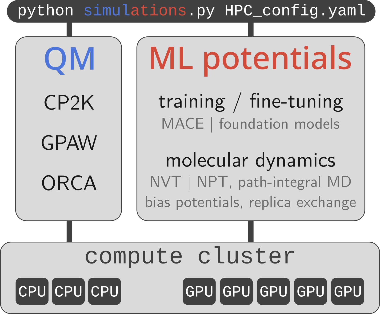
quantum mechanical calculations at various levels of theory (GGA and hybrid DFT, post-HF methods such as MP2 or RPA, and even coupled cluster; using CP2K | GPAW | ORCA)
-
trainable interaction potentials as well as easy-to-use universal potentials, e.g. MACE-MP0
- a wide range of sampling algorithms: NVE | NVT | NPT, path-integral molecular dynamics, alchemical replica exchange, metadynamics, phonon-based sampling, thermodynamic integration; using i-PI, PLUMED, ...
Users may define arbitrarily complex workflows and execute them automatically on local, HPC, and/or cloud infrastructure. To achieve this, psiflow is built using Parsl: a parallel execution library which manages job submission and workload distribution. As such, psiflow can orchestrate large molecular simulation pipelines on hundreds or even thousands of nodes.
FAQ
Where do I start?
Take a brief look at the examples or walk through the documentation to get an idea for psiflow's capabilities. Next, head over to the setup & configuration section of the docs to get started!
Is psiflow a workflow manager?
Absolutely not! Psiflow is a Python library which allows you to perform complex molecular simulations and scale them towards large numbers of compute nodes automatically. It does not have 'fixed' workflow recipes, it does not require you to set up 'databases' or 'server daemons'. The only thing it does is expose a concise and powerful API to perform arbitrarily complex calculations in a highly efficiently manner.
Is it compatible with my cluster?
Most likely yes. Check which resource scheduling system your cluster uses (probably either SLURM/PBSPro/SGE). If you're not sure, ask your system administrators or open an issue
Can I use VASP with it?
You cannot automate VASP calculations with it, but in 99% of cases there is either no need to use VASP, or it's very easy to quickly perform the VASP part manually, outside of psiflow, and do everything else (data generation, ML potential training, sampling) with psiflow. Open an issue if you're not sure how to do this.
I would like to have feature X
Psiflow is continuously in development; if you're missing a feature feel free to open an issue or pull request!
I have a bug. Where is my error message and how do I solve it?
Psiflow covers essentially all major aspects of computational molecular simulation (most notably including the executation and parallelization), so there's bound to be some bug once in a while. Debugging can be challenging, and we recommend to follow the following steps in order:
- Check the stderr/stdout of the main Python process (i.e. the
python main.py
   config.yaml
one). See if there are any clues. If it has contents which you don't understand, open an issue. If there's seemingly nothing there, go to step 2. - Check Parsl's log file. This can be found in the current working directory, under
psiflow_internal/parsl.log. If it's a long file, search for any errors usingErrororERROR. If you find anything suspicious but do not know how to solve it, open an issue. - Check the output files of individual ML training, QM singlepoints, or i-PI molecular
dynamics runs. These can be found under
psiflow_internal/000/task_logs/*. Again, if you find an error but do not exactly know why it happens or how to solve it, feel free to open an issue. Most likely, it will be useful to other people as well - Check the actual 'jobscripts' that were generated and which were submitted to the
cluster. Quite often, there can be a spelling mistake in e.g. the compute project you
are using, or you are requesting a resource on a partition that is not available.
These jobscripts (and there output and error) can be found under
psiflow_internal/000/submit_scripts/.
Where do these container images come from?
They were generated using Docker based on the recipes in this repository, and were then
converted to .sif format using apptainer
Can I run psiflow locally for small runs or debug purposes?
Of course! If you do not provide a config.yaml, psiflow will just use your local
workstation for its execution. See e.g. this or this config used for testing.
Citing psiflow
Psiflow is developed at the Center for Molecular Modeling. If you use it in your research, please cite the following paper:
Machine learning Potentials for Metal-Organic Frameworks using an Incremental Learning Approach, Sander Vandenhaute et al., npj Computational Materials, 9, 19 (2023)