User Guide¶

Deriving a force field from ab initio input consists of several steps. First, one should first configure the QuickFF run. This configuration includes all settings regarding input/output, the force field energy expression and the applied algorithms. This is done by means of the Settings module. A settings instance is constructed by the qff.py script and should also be constructed when using QuickFF as a library. Furthermore, QuickFF can be used in two ways: by means of a single command using the qff.py script or by importing it as a Python library in an external script. This guide elaborates on all these aspects.

QuickFF Settings¶

The configuration parameters for the construction of the force field are stored in an instance of the Settings class. These configuration settings include:

Configuration of the logger
File names for input (eg. the Yaff parameter file for the electrostatic contribution) and output (eg. the Yaff parameter file for the covalent force field, system file, trajectory file, …)
Settings for the non-bonding contributions (eg. cutoff)
Settings specifying the energy expression of the covalent force field (do_bonds, do_bends, do_dihedrals, do_oopdists, bond_term, bend_term, do_squarebend, …)
Settings to finetune the fitting algorithms (do_hess_mass_weighting, cross_svd_rcond, …)

These settings can be specified by either of the following means:

the system-wide default settings defined in the config file quickffrc in the share directory.
a QuickFF config file specified using the --config keyword argument of qff.py or directly to the Settings constructor in a custom written script
keyword arguments given to qff.py or the Settings constructor in a custom written script

Defining options using a keyword arguments overwrites a custom config file as well as the quickffrc file and the settings from a custom config file overwrite the default file quickffrc.

Settings description¶

In this section, a list is included of all settings that can be configured using the Settings routine, either by an entry in the configuration file (CF) denoted in italics or by a keyword arguments (KA) denoted like this. The default value for each setting is given in the quickffrc file (see below). If you are looking for the meaning of a specific setting in the config file, use the search function of this web site.

General settings¶

Logging level (CF: log_level, KA: see description below):
Defines the level of logging of the progress of a QuickFF run. Four possible levels are implemented, which can be defined in CF by means of the string name or the corresponding integer. Some logging levels can also be specified using the corresponding keywork arguments given between paranthesis.
0, silent (--silent): logging is completely switched off

1, low: minimal logging

2, medium: default logging level, logs on what part of the run is currently processed without including any details.

3, high (--verbose): more details in the logging output, includes the force field parameters after each step in the parameterization protocoll.

4, highest (--very-verbose): logging on every detail, usefull for debugging purposes. Includes detailed progress on the construction of the perturbation trajectories.
Logging file (CF: log_file, KA: --logfile):

Defines the name of file were to write the logging output to. Defaults to the standard output (i.e. the screen).
Program mode (CF: program_mode, KA: --program-mode):
Specify the program to execute during the run. The following programs are currently supported:
- MakeTrajectories:
  
  construct the perturbation trajectories and write them to a file for later post-processing. Can be usefull if one intends to generate various force fields using different settings, but all require the same perturbation trajectories. Requires the specification of a non-existing file name for the Perturbation trajectory file name (see further).
- PlotTrajectories:
  
  plot the energy contribution along the given perturbation trajectory. Requires the specification of an existing file name for the Perturbation trajectory file name (see further).
- DeriveFF:
  
  Complete run to construct a force field. This is the default.

Input/output settings¶

Yaff file name (CG: fn_yaff, KA: --fn-yaff):

File name for the Yaff parameter file containing the parameters of the covalent fitted force field. Default is pars_yaff.txt.
CHARMM parameter file (CF: fn_charmm22_prm, KA: N/A):

File name to write the covalent force field parameters to in CHARMM format. Defaults to None, i.e. no such file is generated.
CHARMM PSF file name (CF: fn_charmm22_psf, KA: N/A):

File name of a PSF file to write the system information to. Can be used in combination with the CHARMM parameter file to perform FF simulations using CHARMM software. Defaults to None, i.e. no such file is generated.
System file name (CF: fn_sys, KA: N/A):

File name for a MolMod CHK file containing the system information. Can be used in combination of a Yaff parameter file to perform FF simulations using Yaff.
Plot trajectories (CF: plot_traj, KA: --plot-traj):

Plot the various energy contributions along the perturbation trajectories. If set to final, plots the various energy contributions along the perturbation trajectories using the final force field. If set to all, plots the contributions along the trajectories using all intermediate force fields (given suffixes _Apt1, _Bhc1, _Cpt2 and _Dhc2) as well as the final force field (given the suffix _Ehc3).
Write XYZ trajectories (CF: xyz_traj KA: --xyz-traj)):

Write the perturbation trajectories in XYZ format.
Trajectory file name (CG: fn_traj, KA: --fn-traj):

Read/write the perturbation trajectories from/to FN_TRAJ. If the given file exists, the trajectories are read from the file. Otherwise, the trajectories are written to the given file.
Only trajectories (CG: only_traj, KA: --only-traj)

Construct the perturbation trajectory only for the terms with the given basenames. This options is only applied in the MakeTrajectories program.

Reference force field contribution settings¶

Electrostatic contribution parameter file (CG: ei, KA: --ei)

Yaff parameter file for the electrostatic contribution.
Electrostatic cutoff (CG: ei_rcut, KA: --ei-rcut)

Real-space cutoff for the electrostatic interactions
Van der Waals contribution parameter file (CG: vdw, KA: --vdw)

Yaff parameter file for the van der Waals contribution.
Van der Waals cutoff (CG: vdw_rcut, KA: --vdw-rcut)

Real-space cutoff for the van der Waals interactions
Residual covalent contribution parameter file (CG: covres, KA: --covres)

Yaff parameter file for the residual covalent contribution.

Force field expression settings¶

Atom types (CG: ffatypes, KA: --ffatypes)

Definition of the atom types. Can either be a list of strings, defining the atom type of each atom in the system. Alternatively, one can also estimate the atom types automatically according to one of the available levels: low, medium, high or highest (see automatic estimation of atom types for more details).
Exclude specific bonds (CG: excl_bonds, KA: N/A)

Exclude specific bond terms from the force field. Specify which terms by giving a list of basenames.
Exclude specific bends (CG: excl_bends, KA: N/A)

Exclude specific bend terms from the force field. Specify which terms by giving a list of basenames.
Exclude specific dihedrals (CG: excl_dihs, KA: N/A)

Exclude specific dihedral terms from the force field. Specify which terms by giving a list of basenames.
Exclude specific out-of-plane distances (CG: excl_oopds, KA: N/A)

Exclude specific out-of-plane terms from the force field. Specify which terms by giving a list of basenames.
Include bonds (CG: do_bonds, KA: N/A)

Boolean to specify whether bond terms are included (possibly appart from the terms specified through excl_bonds).
Include bends (CG: do_bends, KA: N/A)

Boolean to specify whether bend terms are included (possibly appart from the terms specified through excl_bends).
Include dihedrals (CG: do_diheds, KA: N/A)

Boolean to specify whether dihedreal terms are included (possibly appart from the terms specified through excl_diheds).
Include out-of-plane distances (CG: do_oops, KA: N/A)

Boolean to specify whether out-of-plane distance terms are included (possibly appart from the terms specified through excl_oopds).
Include Angle-pattern Stretch-Stretch cross terms (CF: do_cross_ASS, KA: N/A):

Include coupling terms between the two stretch terms (i.e. the bonds) featuring in an angle term. In other words, the coupling between neighboring bond terms.
Include Angle-pattern Stretch-Angle cross terms (CF: do_cross_ASA, KA: N/A):

Include coupling terms between an angle term and its constituting bond terms.
Include Dihedral-pattern Stretch-Stretch cross terms (CF: do_cross_DSS, KA: N/A):

Include coupling terms between the two outer stretch terms (i.e. the bond lengths) featuring in an dihedral term. In other words, the coupling between bond terms that are seperated by one other bond.
Include Dihedral-pattern Stretch-Dihedral cross terms (CF: do_cross_DSD, KA: N/A):

Include coupling terms between an outher stretch (i.e. a bond length) in a dihedral and the dihdral angle.
Include Dihedral-pattern Angle-Angle cross terms (CF: do_cross_DAA, KA: N/A):

Include coupling terms between the two angles terms in a dihedral term.
Include Dihedral-pattern Angle-Dihedral cross terms (CF: do_cross_DAD, KA: N/A):

Include coupling terms between an bending angle in a dihedral pattern and the corresponding dihedral angle.
Potential for bond terms (CF: bond_term, KA: N/A)
Specify the functional form of the bond potential. Can be one of the following possibilities:
- bondharm: harmonic potential
  
  $V(r)=\frac{K}{2}\left(r-r_0\right)^2$
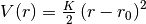
- bondfues: Fues potential, i.e. harmonic in $\frac{1}{r}$
  
  $V(r)=\frac{K}{2}\left(\frac{1}{r}-\frac{1}{r_0}\right)^2$
- bondmm3: the anharmonic bond potential from the MM3 force field ( $\alpha=2.55 \text{\AA}^{-1}$ )
  
  $V(r)=\frac{K}{2}\left(r-r_0\right)^2\left[1-\alpha\left(r-r_0\right)+\frac{7}{12}\alpha^2\left(r-r_0\right)^2\right]$
Potential for bend terms (CF: bend_term, KA: N/A)
Specify the functional form of the bend potential. Can be one of the following possibilities:
- bendharm: harmonic potential
  
  $V(r)=\frac{K}{2}\left(r-r_0\right)^2$
- bendmm3: the anharmonic bend potential from the MM3 force field
  
  $V(r)=\frac{K}{2}\left(\theta-\theta_0\right)^2\left[1-\alpha_1\left(\theta-\theta_0\right)+\alpha_2\left(\theta-\theta_0\right)^2-\alpha_3\left(\theta-\theta_0\right)^3+\alpha_4\left(\theta-\theta_0\right)^4\right]$
  
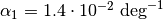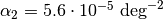  $\alpha_1=1.4\cdot 10^{-2}\ \text{deg}^{-1}$ , $\alpha_2=5.6\cdot 10^{-5}\ \text{deg}^{-2}$ , $\alpha_3=7.0\cdot 10^{-7}\ \text{deg}^{-3}$ and $\alpha_4=2.2\cdot 10^{-8}\ \text{deg}^{-4}$
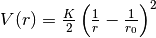
Convert angle to SquareBend term (CF: do_squarebend, KA: N/A)

Identify bend patterns in which 4 atoms of type A surround a central atom of type B with A-B-A angles of 90/180 degrees. A simple harmonic pattern will not be adequate since a rest value of 90 and 180 degrees is possible for the same A-B-A term. Therefore, a cosine term with multiplicity of 4 is used (which corresponds to a chebychev4 potential with sign=-1):

$V\left(\theta\right)= \frac{K}{2}\left[1-\cos\left(4\theta\right)\right]$

To identify the patterns, it is assumed that the rest values have already been estimated from the perturbation trajectories. For each master and slave of a BendAHarm term, its rest value is computed and checked if it lies either the interval [90-threshold ,90+threshold ] or [180-threshold ,180]. If this is the case, the new cosine term is used (the threshold is set to 20 degrees in the routine do_squarebond routine)
Convert angle to BendCLin term (CF: do_bendclin, KA: N/A)

No Harmonic bend can have a rest value equal that is larger than 180° - threshold . If a master (or its slaves) has such a rest value, convert master and all slaves to BendCLin (which corresponds to a chebychev1 potential with sign=+1).
Convert SquareOopdist to Oopdist (CF: do_sqoopdist_to_oopdist, KA: N/A)

Transform a SqOopdist term with a rest value that has been set to zero, to a term Oopdist (harmonic in Oopdist instead of square of Oopdist) with a rest value of 0.0 A.

Fitting algorithm settings¶

Mass Weighting (CF: do_hess_mass_weighting, KA: N/A):

Set to True to apply mass weighting to the Hessian before fitting force constants.
Project negative frequencies (CF: do_hess_negfreq_proj, KA: N/A)

Set to True to project possible negative frequencies out of the ab initio hessian prior to fitting force constants
Singular Value Decomposition for cross terms (CF: do_cross_svd, KA: NA/)

Set to True to perform a singular value decomposition of the cost function to fit the force constants of the cross terms. Singular values that are to smaller than rcond times the largest singular value are filtered out. The value of rcond can be specified with the setting cross_svd_rcond.
Rcond of the SVD for cross terms (CF: cross_svd_rcond, KA: N/A)

See description of the setting do_cross_svd for more info.
Convergence tolerance for perturbation trajectories (CF: pert_traj_tol, KA: N/A)

Convergence criteria for the construction of the perturbation trajectory.
Noise level for error estimation for perturbation trajectories (CF: pert_traj_energy_noise, KA: N/A)

If a float is given, this value is used to perform an error estimation of the force field parameters derived from the perturbation trajectories. Such error estimation is done by repeating the parabolic fitting step multiple times, each time after adding random noise to the energy values (normally distributed with a mean of zero and an standard deviation given by the value defined by this setting). If the resulting error on the newly fitted force field parameters is found to be too high, these parameters are ignored and instead the previous value is reused (or a force constant of zero and rest value from the equilibrium structure if this error was in the first QuickFF step). Furthermore, a warning of such modification is logged if the log level is 3 or higher (with a log level of 4, a full error summary will be given for all parameters). If this setting is set to None, no such error estimation will be performed. To define a value of 0.01 kJ/mol, just write 0.01*kjmol.

Default settings¶

As mentioned before the default settings are defined in the file quickffrc in the share directory. The content if this file is given below.

#IO
fn_yaff                 :   pars_yaff.txt
fn_charmm22_prm         :   None
fn_charmm22_psf         :   None
fn_sys                  :   system.chk
plot_traj               :   None
xyz_traj                :   False
fn_traj                 :   None
log_level               :   medium
log_file                :   None

#Program
program_mode            :   DeriveFF

#FF config
only_traj               :   PT_ALL
ffatypes                :   None
ei                      :   None
ei_rcut                 :   None #default is 20 (periodic) or 50 (non-per) A
vdw                     :   None
vdw_rcut                :   20*angstrom
covres                  :   None

excl_bonds              :   None
excl_bends              :   None
excl_dihs               :   None
excl_oopds              :   None

do_hess_mass_weighting  :   True
do_hess_negfreq_proj    :   False
do_cross_svd            :   True
pert_traj_tol           :   1e-3
pert_traj_energy_noise  :   None
cross_svd_rcond         :   1e-8

do_bonds                :   True
do_bends                :   True
do_dihedrals            :   True
do_oops                 :   True
do_cross_ASS            :   True
do_cross_ASA            :   True
do_cross_DSS            :   False
do_cross_DSD            :   False
do_cross_DAA            :   False
do_cross_DAD            :   False
consistent_cross_rvs    :   True
remove_dysfunctional_cross : True

bond_term               :   BondHarm
bend_term               :   BendAHarm

do_squarebend           :   True
do_bendclin             :   True
do_sqoopdist_to_oopdist :   True

Preparing electrostatic force field¶

A Yaff force field file for the electrostatic contribution can be constructed from the output of HORTON using the qff-input-ei.py script:

qff-input-ei.py [options] fn_sys fn_wpart:path

Arguments

fn_sys

a file containing the system information. Any file type accepted by the main script qff.py is also accepted here (see input files).
fn_wpart

is a HORTON: HDF5 file containing the charges of each atom. The script horton-wpart.py derives atomic charges from wavefunction files and writes the results in this type of HDF5 file. The charges in this file should have the same ordering as the atoms in the system file fn_sys.
path

is the path in the HDF5 to the dataset charges. The default path in HORTON 2.x is /charges. In HORTON 1.x, the path depends on the method used to compute the charges, e.g. /wpart/hi/charges would be the path to the Hirshfeld-I charges.

Options

Force field atom types (--ffatypes=LEVEL):

Determine the force field atom types according to the given level (see automatic estimation of atom types). By default, the atom types are assumed to be defined in fn_sys.
Gaussian distributed charges (--gaussian):

Treat the atomic charges as Gaussian charge distributions with atomic radii determined according to the precedure of Chen et al., implemented in the routine get_ei_radii from the tools module.

Remarks

All electrostatic interactions will be included in the force field, i.e. no scaling is applied. This means that atoms that are connected to each other 1, 2 or 3 bonds will also interact electrostatically. To change this behaviour, open the resulting Yaff parameter file after applying this script, and change the corresponding scales in the file. For example: FIXQ:SCALE 1 0.0 will turn of electrostatic interactions for bonded atoms. See also the Yaff page on the parameter file for electrostatic interactions.

The script might print a WARNING to the screen indicating the for a certain atom type the standard deviation of the charges for this atom type is rather high. This could indicate that the current atom types are to general, i.e. not specific enough for the current chemical configuration. A higher level of atom type specification might then be adequate.

QuickFF main script qff.py¶

The most straightforward use of QuickFF is by means of a single command using the qff.py script. The basic usage of this script is as follows:

qff.py [options] fns

In the sections below, both the input files and the optional arguments are discussed in detail. The description below is further illustrated with examples in the tutorials.

Mandatory input files¶

The script requires input files describing the system and reference data. These files are provided to the program by means of the mandatory arguments fns which should be the names of the files in question. If multiple files, information in later files overwrites information from earlier files. The following list enumerates all possible formats of these input files:

Gaussian formatted checkpoint file (file.fchk):

a file generated using the formchk utility on a checkpoint file from a Gaussian freq job. The atomic numbers, equilibrium geometry and equilibrium Hessian are extracted from this file.
vasprun file (vasprun.xml):

an XML file generated by VASP during a frequency calculation.
MolMod checkpoint file (file.chk)
a file generated the molmod.io.chk.dump method from MolMod. This file contains arrays representing data stored in a computer-friendly format. Each array is stored in the following format:
tag kind=dtype shape datanumber1 datanumber2 datanumber3 datanumber4 datanumber5 datanumber6 datanumber7 datanumber8 ...
QuickFF will recognize and read arrays with the following tags: energy, grad(ient), hess(ian), pos (or coords), rvecs (or cell), bonds, ffatypes and ffatype_ids

Optional input files¶

Electrostatic contribution (--ei=EI):

The user can define the electrostatic contribution of the force field using the option --ei=EI. EI should be the file name of a Yaff parameter file containing the electrostatic contribution. Such a parameter file can be generated. from a HDF5 file containing charges using the script qff-input-ei.py.
Van der Waals contribution (--vdw=VDW):

The user can define the van der Waals contribution of the force field using the option --vdw=VDW. VDW should be the file name of a Yaff parameter file containing the van der Waals contribution.
Residual covalent contribution (--covres=COVRES):

The user can define an a priori defined contribution to the covalent force field (and build a quickff force field on top of it) using the option --covres=COVRES. QuickFF will not neglect terms already present in the residual contribution, instead it will add an extra term for it. COVRES should be the file name of a Yaff parameter file containing the residual terms.

Automatic estimation of atom types¶

The optional argument --fflevel=LEVEL will trigger the automatic assignation of atom types to every atom in the system. There are four possible levels of assignation:

low: atom type is based on atom number

medium: atom type is based on atom number and number of neighbors.

high: atom type is based on atom number, number of neighbors and the atom number of those neighbors.

highest: every single atom is given a unique atom type based on its index in the system.

The levels medium and high are the most usefull, medium will result in higher transferability of the force field parameters, while high will result in higher accuracy. The levels low and highest are mostly usefull for debugging purposes. The automatic assignation for the levels medium and high is illustrated for three different molecules in the figures below. If the level medium is chosen, atom type strings will be of the form EN in which E is the element and N is the number of neighbors. When choosing atom types according to the level high, atom type strings will be of the form ENs in which E is the element, N is the number of neighbors and s is a string describing the neighbors. If the atom has only 1 neighbor, then s is equal _e with e the element of the neighbor. If the atom under consideration has 2 neighbors, then s is equal to _ee in which the first and second e represent the element of the first and second neighbor respectively. If the atom has more than 2 neighbors, then s will contain a substring _en for every neighboring atom. In this substring, e represents the neighbor element and n is the number of neighbors of that particular neighbor element. Multiple instances of this _en string are ordered according to atomic number.

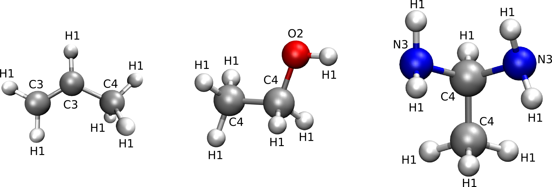
Figure 1: Medium-level atom types

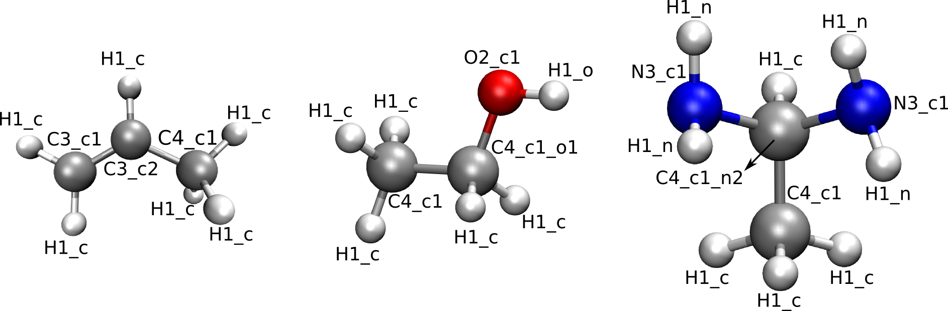
Figure 2: High-level atom types

By default, the automatic assignation is switched off and the atom types are suposed to be defined in the input files.

Miscellanous options¶

Through the use of the following options, the user can manipulate what QuickFF will exactly do.

Program mode (-m PROGRAM_MODE or --program-mode=PROGRAM_MODE):

Specify the program mode which defines the set of instructions that will be executed. Allowed strings are the names of the program classes defined in the program module. Be carefull, these names are case sensitive. By default, the program DeriveNonDiagFF will be used.
Trajectory storing/loading (--fn-traj=FN_TRAJ):

Depending if the given option argument corresponds to an existing file or not, this option will load/save perturbation trajectories to/from a cPickled file.
Construct specific trajectories (--only-traj=ONLY_TRAJ):

Construct the perturbation trajectory only for the terms with the given basenames. This options is only applied in the MakeTrajectories program.
Output file suffix (--suffix=SUFFIX):

Suffix that will be added to all output files. By default, no suffix is added.
Plot energy (-e or --ener-traj):

Plot the various energy contributions along the perturbation trajectories to. By default, energy plotting is switched off.
Dump trajectories in XYZ format (-x or --xyz-traj):

Dump the perturbation trajectories in XYZ format. By default, trajectory dumping is switched off.

Output¶

During the derivation of the force field, QuickFF will dump some usefull information to the screen including machine information, system information, model information, the force field parameters after the perturbation step and the final force field parameters. Additionally, three output files are generated:

system.chk:

A MolMod checkpoint file containing all system information. This file can be used to start new QuickFF calculations or to perform force field simulations using Yaff together with the file pars_yaff.txt.
pars_yaff.txt:

A formatted text file defining the final force field. This file can be read by Yaff together with the file system.chk, to perform force field simulations.

Logging¶

These options control the logging of all the operations in QuickFF.

Silent mode (-s or --silent):

Swith of all logging completely, overwrites all other verbosity options. By default, the silent mode is not activated.
Verbose mode (-v or --verbose):

Increases verbosity, is overwriten if --silent or --very-verbose is switched on. By default, the verbose mode is not activated.
Very verbose mode (-V or --very-verbose):

Increases verbosity to highest level, is overwriten if --silent is switched on. This is mostly usefull for debugging purposes. By default, the very verbose mode is not activated.
Pipe logging (-l LOGFILE or --logfile=LOGFILE):

Redirect logger output to a file with the name LOGFILE. By default, all logging output is printed to the screen.

Parallel QuickFF¶

If Scoop is installed, it is possible to run QuickFF on multiple cores of a single node by using the optional argument --scoop. Only the generation of the perturbation trajectories will be parallized as it is the slowest step. The exact syntax to use QuickFF in parallel is:

python -m scoop -n nproc /path/to/qff.py --scoop [options] fns

nproc is the number of processes that can be launched simultaneously. It is important to note that one has to define the absolute path to the location of the qff.py script. Finally, [options] and fns have the same meaning as in the serial version.

WARNING: There might occur an error (concerning __reduce_cython__) when running QuickFF in parallel with SCOOP. We are aware of this and are looking to solve it in a future release. This can be the case when using Scoop v0.7 or higher.

Importing QuickFF as a library¶

QuickFF can also be treated as library of classes and methods that is imported in a script written by the user. This procedure allows more control over the core features of QuickFF and also allows more complex force fields. In this User Guide, we will show how to write a custom script for deriving a force field using QuickFF. The tutorials will include examples of specific systems, such as water and biphenyl.

Define the system¶

First we need to define an instance of the Yaff System class to define the molecular system:

from molmod.units import angstrom
from yaff import System
import numpy as np
#initialize system
numbers = np.array([1,1])
coords = np.array([[-0.37*angstrom,0.0,0.0],[0.37*angstrom,0.0,0.0]])
system = System(numbers, coords, rvecs=None)

Here, we considered a (non-periodic) hydrogen molecule oriented along the x-axis and a H-H bond length of 0.74 angstrom.

Define the ab initio reference¶

Second, we define the ab initio geometry, gradient and Hessian in equilibrium:

from quickff.reference import SecondOrderTaylor
#initialize numpy arrays
energy = 0.0
grad = np.zeros([2,3], float)
hess = np.zeros([...], float)
#initialize the ab initio reference
ai = SecondOrderTaylor('ai', coords=coords, energy=energy, grad=grad, hess=hess)

Define force field reference objects¶

Next, we define an extra reference object for each force field reference we want to include. Suppose we want to take an a priori derived electrostatic contribution into account. If a Yaff parameter file pars_ei.txt is at hand for the EI contribution, we can add it as follows:

from yaff.pes.ff import ForceField
from quickff.reference import YaffForceField
ff = ForceField.generate(system, 'pars_ei.txt', rcut=10*angstrom)
ei = YaffForceField('ei', ff)

The keyword argument rcut represents the cutoff for the electrostatic interactions, which was given a high enough value to include all interactions of our gas-phase system. Instead of reading the electrostatic force field (ff in the code block above) from a given parameter file, one can also define it using Yaff as a library. For more information see page in the Yaff manual on Beyond force field parameter files.

Define the program and run it¶

Finally, one has to define a program, which is a sequence of routines of the BaseProgram class (see Reference Guide for more information). For our example of a single hydrogen molecule, one could get an accurate estimate of both the bond rest value and its force constant from the perturbation trajectories without force constant refinement:

from quickff.program import BaseProgram
class CustomProgram(BaseProgram):
    def run(self):
        self.do_pt_generate()
        self.do_pt_estimate()
        self.make_output()

program = CustomProgram(system, ai, ffrefs=[ei])
program.run()

The arguments of the initializer of CustomProgram, both mandatory and keyword arguments, are the same as the BaseProgram class (see Reference Guide for more information).

Logging¶

Controlling the amount of logging can be done at the beginning of your custom script as follows:

from quickff.log import log
log.set_level(level)

In the second line of code, level should be either the string silent, low, medium, high or highest, or an integer withing the range 0-4 (0 corresponds to silent, 4 corresponds to highest). One can introduce custom logging sections in the script as follows:

with log.section(key, print_level, timer=timer_description):
    #insert code here
    ...
    #dump string to logger
    log.dump(string)

The meaning of the various variables is:

key: A short description of the section. This will be repeated in the begining of each line dumped to the logger under that section.
print_level: the minimum level that should be assigned to the logger (through the use of log.set_level) to actually print the strings passed through log.dump.
timer_description: The description of this section that will be used in the timings of each section. If None is given, no timing will be included for this section.
string: a string that will be dumped to the logger

For example, the code below:

with log.section('TEST', 2, timer='Testing the logger'):
    log.dump('This is a test')

will generate the following line in the log output if log.level is set to medium or higher:

TEST   This is a test

and the following line at the end of the log output (actual timing below is not representative):

TIMING Testing the logger              0:00:00.000001