2. The back-propagation algorithm for the computation of energy derivatives¶

2.1. Introduction¶

The implementation of partial derivatives of the potential energy towards Cartesian coordinates, uniform scalings (virial), partial charges, inducible dipoles, and so on, can become rather tedious when the potential has a complicated functional form. This chapter describes an implementation strategy that brings the fun back in coding partial derivatives, even when the functional form is complicated. The discussion is limited to first-order partial derivatives, but generalizations of the same idea towards higher-order derivatives are possible. The idea is taken from the field of neural networks and is casted in a form that makes sense for molecular mechanics models. In analogy with neural networks, the same technique can be used to compute derivatives of the energy towards force-field parameters, which may be useful for the calibration of parameters.

No knowledge about neural networks is required to understand the algorithm. Basic knowledge of multidimensional functions, the chain rule and the Jacobian transformation are sufficient. The examples are written in Python and use the Numpy library for array operations. It is assumed that the Numpy library is imported as follows:

import numpy as np

2.2. Abstract example¶

Consider the following function of a vector \(\mathbf{x}\):

\[e(\mathbf{g}(\mathbf{f}(\mathbf{x})), \mathbf{h}(\mathbf{x}))\]

The functions \(\mathbf{f}\), \(\mathbf{g}\) and \(\mathbf{h}\) take vectors as input and produce vectors as output. The function \(e\) takes two vectors as input and produces a scalar as output. The sizes of all vectors are not essential and can all be different. For the sake of completeness, they are defined as follows:

\[ \begin{align}\begin{aligned}\mathbf{x} \in \mathbb{R}^{N_x}\\\mathbf{f}(\mathbf{x}) \in \mathbb{R}^{N_f}\\\mathbf{g}(\mathbf{f}(\mathbf{x})) \in \mathbb{R}^{N_g}\\\mathbf{h}(\mathbf{x}) \in \mathbb{R}^{N_h}\end{aligned}\end{align} \]

We want to obtain a straight-forward and easily verifiable implementation of the function \(e\) and its first-order derivatives towards the components of the vector \(\mathbf{x}\). This can be achieved by implementing the complicated function \(e(x)\) in separate steps and by applying the same decomposition to the computation of the partial derivatives.

The forward code path implements the evaluation of \(e(x)\) as follows:

Compute \(\tilde{\mathbf{f}} = \mathbf{f}(\mathbf{x})\)
Compute \(\tilde{\mathbf{h}} = \mathbf{h}(\mathbf{x})\)
Compute \(\tilde{\mathbf{g}} = \mathbf{g}(\tilde{\mathbf{f}})\)
Compute \(\tilde{e} = e(\tilde{\mathbf{g}}, \tilde{\mathbf{h}})\)

From a mathematical perspective, nothing new is achieved, like it should. From the programming perspective, this breakdown is actually different. This can be seen by coding up both approaches in python:

# The following functions are ingredients for the two examples below.
# The actual code inside these functions is not essential and
# represented by the ``function.foo.of.vector.bar`` stubs.

def vector_fn_f(vector_x):
    '''takes vector x as input, returns vector f(x)'''
    return function.f.of.vector.x

def vector_fn_g(vector_f):
    '''takes vector f as input, returns vector g(f)'''
    return function.g.of.vector.f

def vector_fn_h(vector_x):
    '''takes vector x as input, returns vector h(x)'''
    return function.h.of.vector.x

def scalar_fn_e(vector_g, vector_h):
    '''takes vectors g and h as input, returns scalar e(g,h)'''
    return function.e.of.vectors.g.h

# Original formulation, nested calls

def g_nested(x):
    return vector_fn_g(vector_fn_f(x))

def e_nested(x):
    return scalar_fn_e(g_nested(x), vector_fn_h(x))

# Formulation broken down in pieces, no nested calls.

def e_flat(x):
    f = vector_fn_f(x)
    h = vector_fn_h(x)
    g = vector_fn_g(f)
    e = scalar_fn_e(g, h)
    return e

The backward code path computes the partial derivatives of the energy towards each intermediate result from the forward code path, in reversed order:

Compute \(\displaystyle g^*_k = \frac{\partial e}{\partial g_k}\) and \(\displaystyle h^*_l = \frac{\partial e}{\partial h_l}\)
Apply the chain rule to compute \(\displaystyle f^*_j = \frac{\partial e}{\partial f_j} = \sum_k \frac{\partial g_k}{f_j} g^*_k\)
Apply the chain rule to compute \(\displaystyle x^*_i = \frac{\partial e}{\partial x_i} = \sum_j \frac{\partial f_j}{x_i} f^*_j + \sum_l \frac{\partial h_l}{x_i} h^*_l\)

where \(x_i\), \(f_j\), \(g_k\) and \(h_l\) are the components of the vectors or vector functions \(\mathbf{x}\), \(\mathbf{f}\), \(\mathbf{g}\) and \(\mathbf{h}\), respectively. When coding the chain rules, one may make use of the sparsity of Jacobian matrix elements instead of using BLAS routines to implement the matrix-vector products in step 2 and 3.

Combined implementation of forward and backward paths. There is an elegant object-oriented way to code both forward and backward paths, such that the forward and backward steps of a single mathematical function, e.g. \(\mathbf{g}(\mathbf{f})\), are tied closely together. The example code below is academic. Real-life code may deviate in terms of style and API deteails. All mathematical functions in this abstract example are implemented as derived class of the Bead class:

class Bead(object):
    # The name `Bead' stresses that each class implements a part of
    # a complete function to which the `Chain'-rule is applied.
    def __init__(self, nins, nout):
        self.nins = nins # list of sizes of the input arrays.
        self.nout = nout # size of the output array
        self.ar_out = np.zeros(nout) # the output of the function
        self.ar_gout = np.zeros(nout) # the derivative of the final scalar
                                      # function towards the outputs

    def forward(self, ars_in):
        '''Subclasses implement a mathematical function here.

           **Arguments:**

           ars_in
                A list of input arrays
        '''
        assert len(self.nins) == len(ars_in)
        for i in range(len(self.nins)):
            assert len(ars_in[i]) == self.nins[i]

    def back(self, ars_gin):
        '''Subclasses implement the chain rule for the mathematical function here.

           **Arguments:**

           ars_gin
                A list of output arrays for the derivatives of the final
                scalar towards the corresponding input arrays of the forward
                method. Results must be added to the arrays ars_gin, not
                overwritten.

           This routine assumes that the contents of self.ar_gout is already
           computed before this routine is called. The code in the subclass
           must transform 'the derivatives of the energy towards the output
           of this function' (self.ar_gout) into 'the derivatives of the
           energy towards the input of this function' (ars_gin).
        '''
        assert len(self.nins) == len(ars_gin)
        for i in range(len(self.nins)):
            assert len(ars_gin[i]) == self.nins[i]

    def resetg(self):
        # clear the gout array
        self.ar_gout[:] = 0

class BeadF(Bead):
    # Imagine some implementations of ``__init__``, ``forward`` and ``back`` methods.
    # The init routine must not have arguments. It may pass fixed input and
    # output sizes to the constructor of the super class.

class BeadG(Bead):
    # Imagine some implementations of ``__init__``, ``forward`` and ``back`` methods

class BeadH(Bead):
    # Imagine some implementations of ``__init__``, ``forward`` and ``back`` methods

class BeadE(Bead):
    # Imagine some implementations of ``__init__``, ``forward`` and ``back`` methods
    # In this case, nout has to be equal to one, because this is a scalar function.

f = BeadF(...) # arugments can be anything, not relevant here
g = BeadG(...)
h = BeadH(...)
e = BeadE(...)

def e_flat(x, gx=None):
    '''When gx is given, it must be an output array for the derivatives of
       e towards the components of the vector x.
    '''
    # forward code path, order does matter
    f.forward([x])
    h.forward([x])
    g.forward([f.ar_out])
    e.forward([g.ar_out, h.ar_out])
    if gx is not None:
       # clear the ar_gout arrays, order does not matter
       e.resetg()
       g.resetg()
       h.resetg()
       f.resetg()
       # backward code path, order does matter
       e.ar_gout[0] = 1 # we now that e is a scalar function
       e.back([g.ar_gout, h.ar_gout])
       g.back([f.ar_gout])
       h.back([gx])
       f.back([gx])
    return e.ar_out[0] # we now that e is a scalar function

The function e_flat can also be represented schematically:

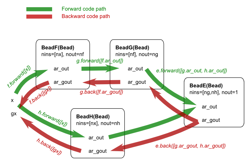
The example above shows that the complexity of the partial derivatives is broken down into smaller pieces that are easier to handle. In fact, this approach has more advantages:

One can envision multiple different implementations of one of the Beads, say BeadG, that can be swapped in and out without having to re-implement the function e_flat. The back-propagation technique chops the computation of the function e and its partial derivatives into orthogonal (in the IT sense) steps.
Each bead can be tested separately with unit tests, see below.

Final remark: the above code could be done with more Python tricks to make the code snappier. This is avoided to make this chapter more accessible to readers with a limited Python background.

2.3. Simple examples of `Bead` subclasses¶

The following two examples are kept as simple as possible. There is nothing exciting about them, yet they completely show how useful the back-propagation may be. With the first two examples, one may implement fully functional neural networks in Python that can compute partial derivatives of the output. Note the use of += in the back methods.

Simple linear transformation plus a constant vector:

class BeadLinTransConst(Bead):
    def __init__(self, coeffs, consts):
        assert len(coeffs.shape) == 2 # must be a transformation matrix
        assert len(consts.shape) == 1 # must be a vector with constants
        assert consts.shape[0] == coeffs.shape[0]
        self.coeffs = coeffs
        self.consts = consts
        Bead.__init__(self, [coeffs.shape[1]], coeffs.shape[0])

    def forward(self, ars_in):
        Bead.forward(self, ars_in)
        self.ar_out[:] = np.dot(self.coeffs, ars_in[0]) + self.consts

    def back(self, ars_gin):
        Bead.back(self, ars_gin)
        ars_gin[0][:] += np.dot(self.coeffs.T, self.ar_gout)

Switching function, tanh, applied to each vector component separately:

class BeadSwitch(Bead):
    def __init__(self, size):
        Bead.__init__(self, [size], size)

    def forward(self, ars_in):
        Bead.forward(self, ars_in)
        self.ar_out[:] = np.tanh(ars_in[0])

    def back(self, ars_gin):
        Bead.back(self, ars_gin)
        # Recycle the intermediate result from the forward computation...
        # This happens quite often in real-life code.
        ars_gin[0][:] += self.ar_gout*(1-self.ar_out**2)

The dot product of two vectors:

class BeadDot(Bead):
    def __init__(self, nin):
        Bead.__init__(self, [nin, nin], 1)

    def forward(self, ars_in):
        Bead.forward(self, ars_in)
        self.ar_out[0] = np.dot(ars_in[0], ars_in[1])
        # keep a hidden reference to the input arrays
        self._ars_in = ars_in

    def back(self, ars_gin):
        Bead.back(self, ars_gin)
        ars_gin[0][:] += self.ar_gout[0]*self._ars_in[1]
        ars_gin[1][:] += self.ar_gout[0]*self._ars_in[0]

These examples are taken from data/examples/999_back_propagation/bp.py in the source tree. That file also contains a completely functional example implementation of a neural network based on the Bead classes.

2.4. Unit testing¶

Each bead may be tested separately, which is a great way of isolating bugs. See data/examples/999_back_propagation/bp.py for practical examples. The unit tests in this example use the generic derivative tester from the molmod module.

2.5. Real example¶

A realistic example, which deviates a little from the Bead API above, can be found in the Yaff source code in the class ForcePartValence in the file yaff/pes/ff.py. This class implements the computation of valence interactions with a minimal amount of code. The back-propagation algorithm plays a crucial role in keeping the code compact.

The computation of the covalent energy is broken into three major beads:

Computation of relative vectors needed for the internal coordinates. See yaff.pes.dlist.DeltaList.
Computation of the internal coordinates based on the DeltaList. See yaff.pes.iclist.InternalCoordinateList.
Computation of valence energy terms (including cross terms) based on the InternalCoordinateList. See yaff.pes.vlist.ValenceList.

Each class has its forward and back methods, which are all implemented in low-level C code for the sake of efficiency. In addition to the benefits mentioned above, this example has some additional specific amenities:

Any internal coordinate can be combined with any functional form of the energy term. Yet, no code was written for each combination.
Cross terms of the form \((x-x_0)(y-y_0)\) are supported for all possible combinations of two internal coordinates, without having to implement all these combinations explicitly.
The Cartesian gradient and virial are computed in the back method of step 1, based on derivatives of the energy towards the relative vectors. This considerably eases the implementation of the virial.

2. The back-propagation algorithm for the computation of energy derivatives¶

2.1. Introduction¶

2.2. Abstract example¶

2.3. Simple examples of `Bead` subclasses¶

2.4. Unit testing¶

2.5. Real example¶

Table Of Contents

Previous topic

This Page

2. The back-propagation algorithm for the computation of energy derivatives¶

2.1. Introduction¶

2.2. Abstract example¶

2.3. Simple examples of Bead subclasses¶

2.4. Unit testing¶

2.5. Real example¶

2.3. Simple examples of `Bead` subclasses¶